Introduction to Scilab Tutorial | Control Systems

Scilab is a free, open-source numerical computation software that is similar to the popular MATLAB. In this tutorial series, we shall see how we can use Scilab to model and simulate concepts in electrical engineering one by one. This will help us to understand concepts more clearly and also solve problems of greater complexity with ease.

In this introductory tutorial we shall see the basics that are required to get started with Scilab. Scilab can be downloaded freely from: http://www.scilab.org/

After it is downloaded and installed, this is how we are welcomed.

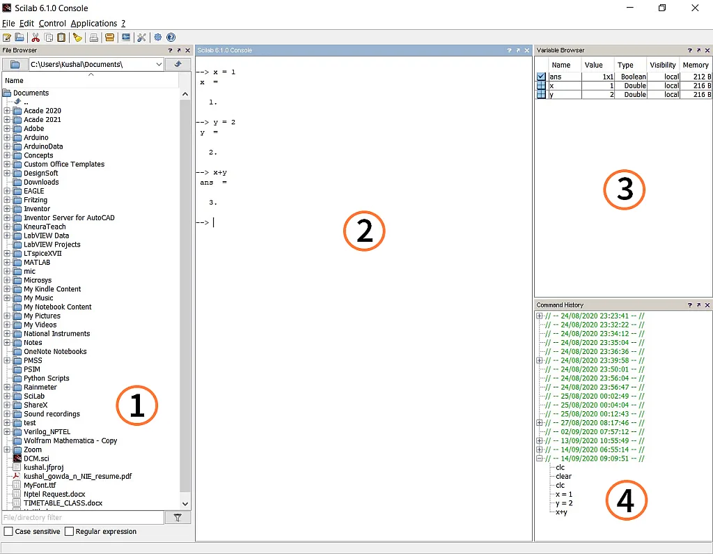
The region marked (1) is the file browser where we choose the folder where we would want to work on, select files and save files. The region marked (2) is the Scilab console or the command window. Here we can just type a command after the prompt that looks like “-->” and the press enter/return to obtain the result of that command. Take a look at the example below.

Here x and y are the variables. If the result of any operation is not assigned to a specific variable, then the result is stored in a temporary variable named “ans” meaning “answer”. So, where do we find all the variables that have been used at one place? It’s the variable browser which is marked (3). To clear the variable browser, just type clear in the console and press enter or return. When your console looks messy, just type clc in the console and press enter / return and it’ll look fresh.

The region marked (4) is the command history. As the name suggests, it keeps a track of all the commands executed.

It is not possible to save commands when we type them into the console window, nor is the console window appropriate to run multiple commands. For this purpose we have the editor window (also called SciNotes) where we can type the commands and save it as a .sce file and then execute it. To open the editor window, go to the top left.

Click on the region marked to open the editor window. It then pops up the window, as shown below.

We’ll use this extensively later but for now, we just wanted to introduce it. Now that we are familiar with the Scilab environment, we shall learn about the basic commands that’ll help you get started with Scilab.

Variables do not need to be declared in Scilab but they must be defined by assigning a value. In case no value is assigned to a variable, then an error pops up.

The names given to variables can be anything except that which is defined by the system.

%pi is constant the is defined by the system which represents π. Let’s have a look at the basic mathematical operations.

We can mask the results from being displayed by using a semicolon (;) and then display it later whenever needed by using the disp() function. We can also just type the name of a variable and press enter / return to display its value.

Vectors and Matrices are defined using square brackets [ ]. While defining them, we use a space or comma to separate the columns and we use a semicolon to separate the rows. Let’s look at the examples of a column vector, a row vector and a matrix.

Now, take a look at these.

We can use the colon operator to create vectors with increments. The first command assigns A to a vector which increments in steps of 1 from 1 to 10 and the second command assigns B to a vector which increments in steps of 3 from 1 to 20.

We also use the colon operator to extract a part of any matrix. Suppose there is a matrix M of order 5x5. Now we would like to extract elements in column 3,4,5 and row 2,3 on to a separate matrix. So how do we do this? Say M_ext is the separate matrix having the extracted elements. We then assign M_ext = M ( 2:3 , 3:5 ). This means that extract elements belonging to row 2 up to row 3 and column 3 up to 5. In another scenario, if we need to extract row 4 of this matrix, then we assign M_ext = M ( 4 , : ). Leaving the either side of the colon empty indicates the console to consider all columns present without restriction. The following examples will make this more clear.

The part of matrix in bold is to be extracted.

The next examples will be very familiar if you have any coding experience. Starting with the If-Else, If-Else statements allow execution of certain commands upon verifying a test case. The examples below will make this clear.

You will see If-Else statements being used much more frequently with SciNotes than using the console.

Select case is a useful alternative to the else-if ladder, it makes our lives easier. Let’s consider the same example as above.

Let’s understand “for” and “while” loops in Scilab by taking a simple example of finding the sum of the first 10 numbers.

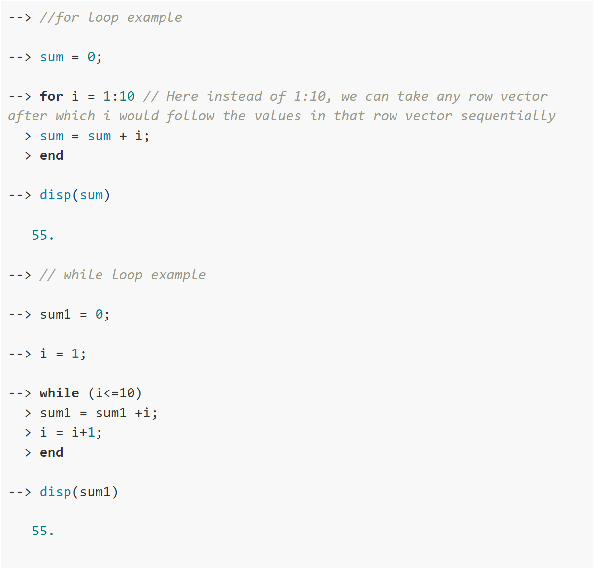
In the “for” loop, commands are executed repeatedly until i takes all the values in the specified range or in the specified row vector. Here, the commands inside the loop are executed repeatedly until i takes all the values from 1 to 10. Whereas in a while loop, commands are executed in a loop after checking a specific condition before each cycle. Here, the commands are repeatedly executed until i becomes more than 10. We obtain the same results using either type of loop, but for loop is preferred in most of the cases.

If a particular operation is to be done again and again, we make it into a function and then call it whenever it is required.

We follow this syntax to define a function.

Inside the function body, we perform operations on input arguments and assign it to the return_variable whose value is returned where the function is called.

Let’s look at the below example.

The function name here is addition and the return variable is y while the input arguments are a and b.

Let’s understand how we can plot graphs in Scilab with the help of the examples below.

And the plot of y = x² is displayed as shown below.

To plot, we must have two equal sized vectors, which should make intuitive sense as they need to show their relationship to each other.

In this tutorial, we understood the basic environment of Scilab, learnt defining variables, and did basic operations on them. Then we understood if-else statements, for - while loops. We then learned how to define functions and how we can use them and, at last, we saw how to plot in Scilab.

With this knowledge, you can start using Scilab for those lengthy calculations in your electrical engineering laboratories. In the upcoming tutorials, we shall be using Scilab to simplify electrical engineering concepts and we shall discuss additional commands as and when required. We shall learn about XCOS, a tool to help us specifically with systems and controls, in the next tutorial.