Root Locus Plot 3.4

Published Jul 06, 2021

In the previous tutorial, we learned about the Routh Hurwitz Criterion and how we can use it to determine the stability of control systems. We also discussed the special cases involved and understood how to use them while designing systems. Moving forward in this chapter on stability, we shall discuss Root Locus Plots in this tutorial. So, what is a root locus plot (or simply just a root locus)? We’ll get there soon. But before that, let’s recall the example that we considered at the end of the last tutorial.

Consider the system with an open-loop transfer function

where K is positive

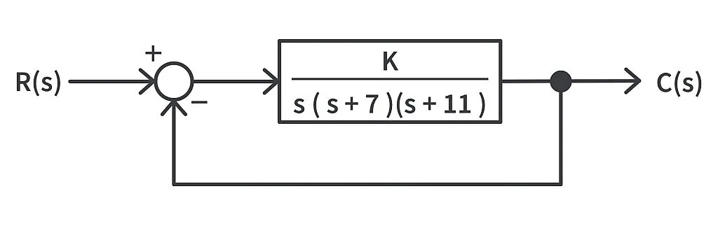
Its closed-loop transfer function is

And the characteristic equation

The constant K here may just represent some constant, but in actual systems, it may be an unknown parameter or a variable parameter and, as we can see in this example, this unknown parameter affects the characteristic equation and in turn affects the location of poles of the system.

To check this, let’s assign a few values to K and then see how the location of poles varies.

As usual, we shall use the help of Scilab for this.

Let’s vary K from 1 to 10000:

s = %s;    // defines 's' as polynomial variable
for k = 1:10000
    tf = syslin('c', k, (s^3 + 18*s^2 + 77*s + k));    
    plzr(tf) //this produces a pole - zero plot of the transfer function tf
end

This will take some time to complete, but you can still observe the location of poles changing. Have a look at this GIF,

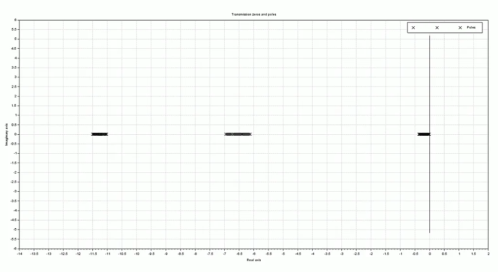
After completion,

As we discussed earlier in chapter 2, the pole locations are responsible for how a system responds. Hence, knowing how the location of poles varies as we vary a certain parameter provides us with a clear picture of what that parameter should be so that the system behaves how we want it to.

Coming back to the root locus, you might have already guessed what a root locus is. It is simply the path that the poles take as we vary a certain parameter. Defining it more formally, the locus of the migration of the roots of the characteristic equation in the s-plane is called root locus.

A ‘for loop’ and a few lines of code did it for us, we shall also see how we can do it in a single step with Scilab later. But how do we do it without computers?

There is a set of 9 rules for the construction of the root locus plot which we shall skip as 1) it is quite overwhelming for a tutorial and 2) it is less used practically. But we shall mention a few essential points.

The first one is the Evans conditions (it was Evan who developed the root locus technique) which form the basis of the root locus.

1. Evans Conditions

Consider a generally closed-loop system as shown,

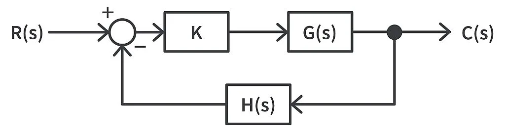
The closed-loop transfer function of the system is given by

As we considered earlier, K is the variable parameter, and we will assume K can vary from

The characteristic equation of the system is given by

As s is a complex variable, we can rewrite the above equation as

This means that for

to be -1 (to be on the real negative axis), it should make an angle of odd multiples of 180°

Comparing both sides of the above equation gives us Evans conditions.

The Magnitude Criterion

Where the magnitude of the open-loop transfer function has to be 1 for each and every point of the root locus

The Angle Criterion

Where the angle of the complex open-loop transfer function at each and every point on the root locus is equal to the odd multiple of 180°

2. The next point is that the root locus is always symmetrical about the real axis.

3. The branches of root locus start at the open-loop poles (at K = 0) and they end at open-loop zeros and if sufficient open-loop zeros are not present, then they end at infinity as in the case of the example earlier. And it is due to this reason that the number of branches that exist in a root locus is equal to the number of open-loop poles. It’s okay if this is confusing, the following examples will make it clear, and we shall discuss it once again with the examples.

Now, with the help of an example, we shall discuss how to plot root locus quickly using Scilab without the traditional looping approach as we did before. With this, we shall also make the points we stated earlier clearer.

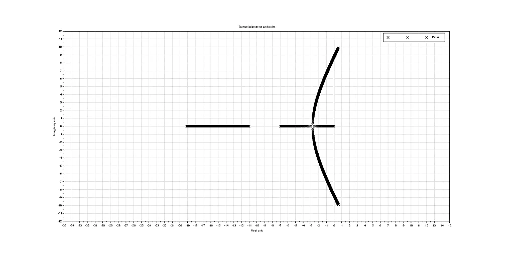
Consider this second-order closed-loop system.

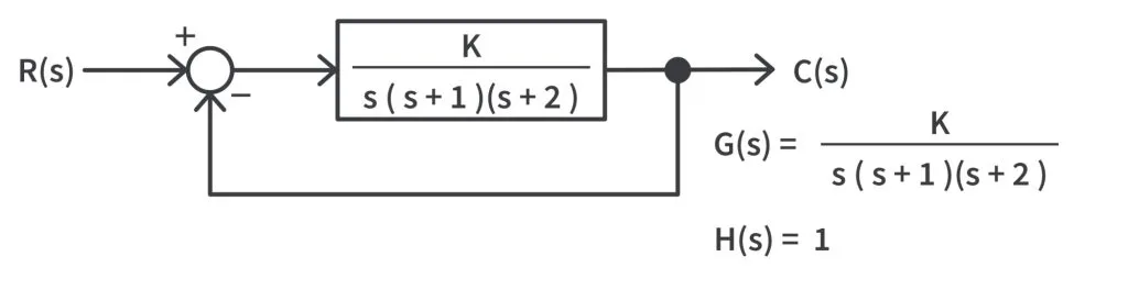
The open-loop transfer function of the system is

The closed-loop transfer function of the system is given by

Have a look at this code below,

s = %s;    // defines 's' as polynomial variable
tf = syslin('c', 1, s*(s+1)*(s+2));    
evans(tf) //this produces the root locus plot of the transfer function tf
mtlb_axis([-5 5 -5 5]) //restricting the axis (Not actually required)

The function used to plot root locus is named after Evans who developed root locus.

One thing that is to be noted is that we always feed in the open-loop transfer function while plotting the root locus and the other thing is that you should replace K with 1 in the open-loop transfer function while plotting the root locus using Scilab.

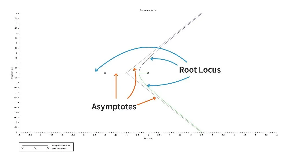
Now, let’s come to the plot we obtained. The asymptotes in the plot just give a rough direction of the root locus.

Observations

The root locus started at 0, -1, -2. This is where the open-loop poles exist, and this justifies the point we made earlier stating that the root locus starts from the open-loop poles.
As there are no open-loop zeros, the root locus ends at infinity.
There are three branches of the root locus marked by black, blue, and green in the plot above. And the three branches are because there are three open-loop poles.

We shall now move further. Say you have a system where you cannot tweak any of the system parameters (consider all the parameters to be fixed), what should we do to tweak the system response to make it more desirable? We need to add a compensator. Have a look at this block diagram.

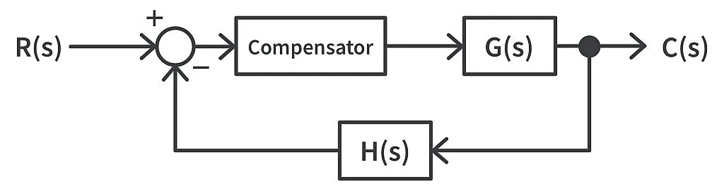
Now the question is - what does this compensator do? It just adds a zero or a pole or both to the existing open-loop system and this addition will help us tweak the root locus and make the system respond closer to the desired response.

Let’s simulate and check.

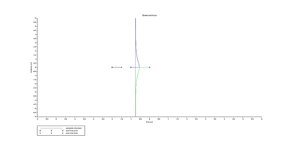
We shall consider that same previous example and we shall add an open-loop pole at various locations and see the changes we obtain in the root locus.

1. Zero at s = -3

So, now the open-loop transfer function becomes

The root locus obtained is

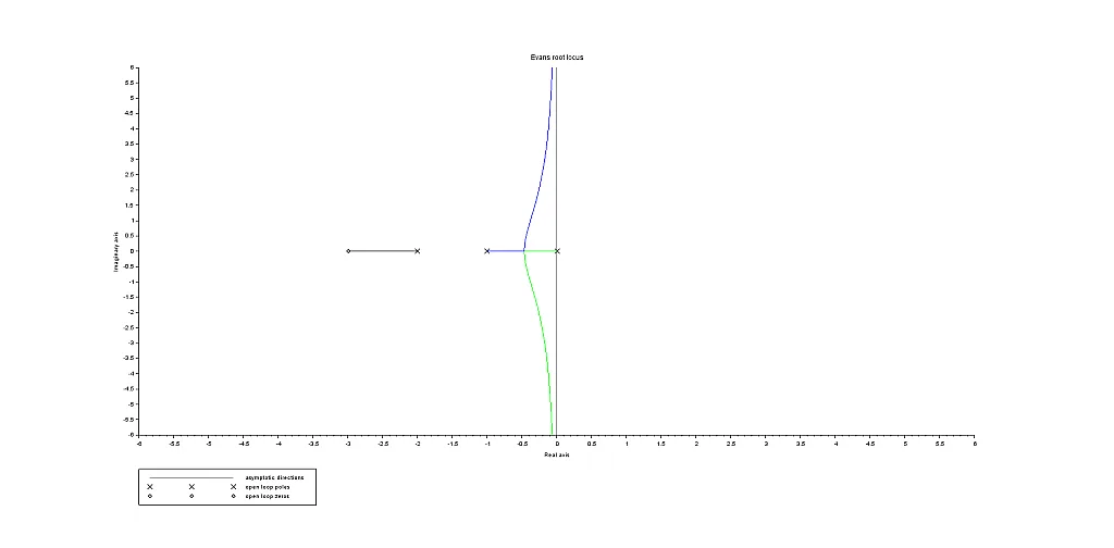
As we discussed, we can see the black coloured branch of the root locus ending at a zero.

2. Zero at s = -1.5

So, now the open-loop transfer function becomes

The root locus,

3. Zero at s = -0.5

So, now the open-loop transfer function becomes

And the root locus,

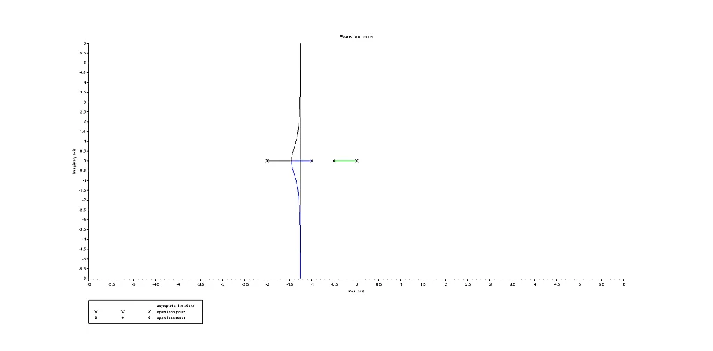
Without an open-loop zero, the root locus of the system existed in the right half of the s plane. Next, by introducing a pole at s = -3, the root locus was reshaped such that the root locus exists only in the left half of s plane and thus making the system stable for all values of K. And then, when we moved the zero from s = -3 to s = -1.5 and then to s = -0.5, the root locus further moved away from the imaginary axis at zero. So, as the open-loop zero moved close to the imaginary axis, the root locus moved toward the left. You can also try adding a pole in a similar way and check its effect on the root locus as an activity. That would have an opposite effect i.e., as the open-loop pole moves closer to the imaginary axis, the root locus would move further toward the right.

What we can conclude is that by using this effect of the addition of zeros and poles on the root locus, we can shape that root locus of a system as we desire. This is the primary purpose of compensators. Although we shall formally start controllers and compensators in the next chapter (also the next tutorial), this should serve as a good introduction on what is the primary purpose of compensators.

In this tutorial, we learned about the root locus plot. We then discussed how to obtain it with the help of Scilab and discussed the observations that we obtain from the root locus plot. In the end, we discussed the effect of the addition of an open-loop pole of zero on the root locus of a system.

With this we come to the end of the third chapter where we started with understanding the basics of stability of control systems and then we discussed the Routh Hurwitz criterion for stability and then we ended it with learning about the root locus. In the next tutorial, we shall start with controllers and compensators. I strongly recommend you try the examples we discussed in this tutorial on Scilab to familiarize yourself further and become more intuitively comfortable with this topic before moving on.

Thank you.

Control Theory (17)
Control Systems (18)

Authored By

Kushal Gowda

An Electrical and Electronics Engineer. Loves playing Table Tennis, Cricket and Badminton . Always ready to learn and teach. His fields of interest include power electronics, e-Drives, control theory and battery systems.

Next up:

Controllers and Compensators | Control Systems 4.1