Digital Communication in the Presence of Noise

When we incorporate additive noise into our channel model, so that

, errors can creep in. If the transmitter sent bit 0 using a BPSK signal set, the integrators' outputs in the matched filter receiver would be:

It is the quantities containing the noise terms that cause errors in the receiver's decision-making process. Because they involve noise, the values of these integrals are random quantities drawn from some probability distribution that vary erratically from bit interval to bit interval. Because the noise has zero average value and has an equal amount of power in all frequency bands, the values of the integrals will hover about zero. What is important is how much they vary. If the noise is such that its integral term is more negative than

, then the receiver will make an error, deciding that the transmitted zero-valued bit was indeed a one. The probability that this situation occurs depends on three factors:

Signal Set Choice — The difference between the signal-dependent terms in the integrators' outputs (equations Equation) defines how large the noise term must be for an incorrect receiver decision to result. What affects the probability of such errors occurring is the energy in the difference of the received signals in comparison to the noise term's variability. The signal-difference energy equals
For our BPSK baseband signal set, the difference-signal-energy term is
$4\alpha^{2}A^{4}T^{2}$ .
Variability of the Noise Term — We quantify variability by the spectral height of the white noise $\frac{N_{0}}{2}$ added by the channel.
Probability Distribution of the Noise Term — The value of the noise terms relative to the signal terms and the probability of their occurrence directly affect the likelihood that a receiver error will occur. For the white noise we have been considering, the underlying distributions are Gaussian. Deriving the following expression for the probability the receiver makes an error on any bit transmission is complicated but can be found at [link] and [link]. 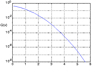$\begin{array}{rcl}p_{e} & = & {Q\left( \sqrt{\frac{\int_{0}^{T}\left( {{s_{1}\left( t \right)} - {s_{0}\left( t \right)}} \right)^{2}d}{2N_{0}}} \right)} \\ & = & {{Q\left( \sqrt{\frac{2\alpha^{2}A^{2}T}{N_{0}}} \right)}\text{~~for\ the\ BPSK\ case}} \\\end{array}$ Here $Q\left( \cdot \right)$ is the integral ${Q\left( x \right)} = {\frac{1}{\sqrt{2\pi}}{\int_{x}^{\infty}e^{- \frac{\alpha^{2}}{2}}d}}$ . This integral has no closed form expression, but it can be accurately computed. As Figure illustrates, is a decreasing, very nonlinear function.

Figure 1. The function Q(x) is plotted in semilogarithmic coordinates. Note that it decreases very rapidly for small increases in its arguments. For example, when x increases from 4 to 5, Q(x) decreases by a factor of 100.

The term

equals the energy expended by the transmitter in sending the bit; we label this term

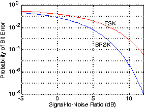
. We arrive at a concise expression for the probability the matched filter receiver makes a bit-reception error.

Figure 2 shows how the receiver's error rate varies with the signal-to-noise ratio

Figure 2. The probability that the matched-filter receiver makes an error on any bit transmission is plotted against the signal-to-noise ratio of the received signal. The upper curve shows the performance of the FSK signal set, the lower (and therefore better) one the BPSK signal set.

Exercise

Derive the probability of error expression for the modulated BPSK signal set, and show that its performance identically equals that of the baseband BPSK signal set.

The noise-free integrator outputs differ by

, the factor of two smaller value than in the baseband case arising because the sinusoidal signals have less energy for the same amplitude. Stated in terms of