Coulomb’s Law

Consider two charge-bearing particles in free space, identified as “particle 1” and “particle 2” in Figure 5.1.1.

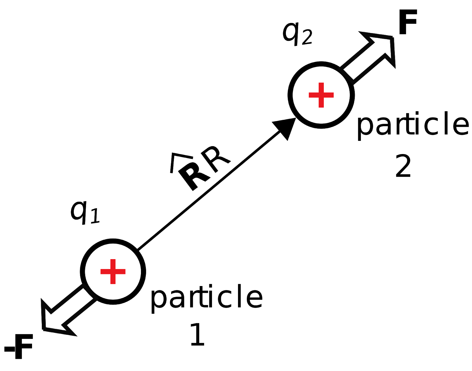
Figure 5.1.1: Coulomb’s Law describes the force perceived by pairs of charged particles.. Image used with permission (CC BY SA 4.0; K. Kikkeri).

Let the charges borne by these particles be

and

, and let

be the distance between them. If the particles bear charges of the same sign (i.e., if

is positive), then the particles repel; otherwise, they attract. This repulsion or attraction can be quantified as a force experienced by each particle. Physical observations reveal that the magnitude of the force is proportional to

, and inversely proportional to

. For particle 2 we find:

where

is the unit vector pointing from the particle 1 to the particle 2, and

is a constant. The value of

must have units of inverse permittivity; i.e., (F/m)

. This is most easily seen by dimensional analysis of the above relationship, including the suspected factor:

where we have used the facts that 1 F

1 C/V, 1 V

1 J/C, and 1 N

1 J/m. This finding suggests that

, where

is the permittivity of the medium in which the particles exist. Observations confirm that the force is in fact inversely proportional to the permittivity, with an additional factor of

(unitless). Putting this all together we obtain what is commonly known as Coulomb’s Law:

Subsequently, the force perceived by particle 2 is equal and opposite; i.e., equal to

Separately, it is known that

can be described in terms of the electric field intensity

associated with particle 1:

This is essentially the definition of

, as explained in Section 2.2. Combining this result with Coulomb’s Law, we obtain a means to directly calculate the field associated with the first particle in the absence of the second particle:

where now

is the vector beginning at the particle 1 and ending at the point to be evaluated.

The electric field intensity associated with a point charge (Equation 5.1.4) is (1) directed away from positive charge, (2) proportional to the magnitude of the charge, (3) inversely proportional to the permittivity of the medium, and (3) inversely proportional to distance squared.

We have described this result as originating from Coulomb’s Law, which is based on physical observations. However, the same result may be obtained directly from Maxwell’s Equations using Gauss’ Law (Section 5.5).

Example 5.4.1: . Electric field of a point charge at the origin.

A common starting point in electrostatic analysis is the field associated with a particle bearing charge

at the origin of the coordinate system. Because the electric field is directed radially away from a positively-charged source particle in all directions, this field is most conveniently described in the spherical coordinate system. Thus,

becomes

becomes

, and we have

Here’s a numerical example. What is the electric field intensity at a distance 1

m from a single electron located at the origin, in free space? In this case,

C (don’t forget that minus sign!),

m, and we find:

This is large relative to electric field strengths commonly encountered in engineering applications. The strong electric field of the electron is not readily apparent because electrons in common materials tend to be accompanied by roughly equal amounts of positive charge, such as the protons of atoms. Sometimes, however, the effect of individual electrons does become significant in practical electronics through a phenomenon known as shot noise.