Filtering in the Frequency Domain
Because we are interested in actual computations rather than analytic calculations, we must consider the details of the discrete Fourier transform. To compute the length-

DFT, we assume that the signal has a duration less than or equal to
. Because frequency responses have an explicit frequency-domain specification in terms of filter coefficients, we don't have a direct handle on which signal has a Fourier transform equaling a given frequency response. Finding this signal is quite easy. First of all, note that the discrete-time Fourier transform of a unit sample equals one for all frequencies. Since the input and output of linear, shift-invariant systems are related to each other by

, a unit-sample input, which has

, results in the output's Fourier transform equaling the system's transfer function.
Exercise
This statement is a very important result. Derive it yourself.
The DTFT of the unit sample equals a constant (equaling 1). Thus, the Fourier transform of the output equals the transfer function.
In the time-domain, the output for a unit-sample input is known as the system's unit-sample response, and is denoted by

. Combining the frequency-domain and time-domain interpretations of a linear, shift-invariant system's unit-sample response, we have that
and the transfer function are Fourier transform pairs in terms of the discrete-time Fourier transform.

Returning to the issue of how to use the DFT to perform filtering, we can analytically specify the frequency response, and derive the corresponding length-
DFT by sampling the frequency response.

Computing the inverse DFT yields a length-
signal no matter what the actual duration of the unit-sample response might be. If the unit-sample response has a duration less than or equal to
(it's a FIR filter), computing the inverse DFT of the sampled frequency response indeed yields the unit-sample response. If, however, the duration exceeds
, errors are encountered. The nature of these errors is easily explained by appealing to the Sampling Theorem. By sampling in the frequency domain, we have the potential for aliasing in the time domain (sampling in one domain, be it time or frequency, can result in aliasing in the other) unless we sample fast enough. Here, the duration of the unit-sample response determines the minimal sampling rate that prevents aliasing. For FIR systems — they by definition have finite-duration unit sample responses — the number of required DFT samples equals the unit-sample response's duration:

.
Exercise
Derive the minimal DFT length for a length-

unit-sample response using the Sampling Theorem. Because sampling in the frequency domain causes repetitions of the unit-sample response in the time domain, sketch the time-domain result for various choices of the DFT length
.
In sampling a discrete-time signal's Fourier transform

times equally over

to form the DFT, the corresponding signal equals the periodic repetition of the original signal.

To avoid aliasing (in the time domain), the transform length must equal or exceed the signal's duration.
Exercise
Express the unit-sample response of a FIR filter in terms of difference equation coefficients. Note that the corresponding question for IIR filters is far more difficult to answer: Consider the example.
The difference equation for an FIR filter has the form

The unit-sample response equals

which corresponds to the representation described in a problem of a length-qq boxcar filter.
For IIR systems, we cannot use the DFT to find the system's unit-sample response: aliasing of the unit-sample response will always occur. Consequently, we can only implement an IIR filter accurately in the time domain with the system's difference equation. Frequency-domain implementations are restricted to FIR filters.
Another issue arises in frequency-domain filtering that is related to time-domain aliasing, this time when we consider the output. Assume we have an input signal having duration

that we pass through a FIR filter having a length-

unit-sample response. What is the duration of the output signal? The difference equation for this filter is

This equation says that the output depends on current and past input values, with the input value

samples previous defining the extent of the filter's memory of past input values. For example, the output at index
figure>
depends on

(which equals zero),

, through

. Thus, the output returns to zero only after the last input value passes through the filter's memory. As the input signal's last value occurs at index

, the last nonzero output value occurs when

or

. Thus, the output signal's duration equals

.
Exercise
In words, we express this result as "The output's duration equals the input's duration plus the filter's duration minus one.". Demonstrate the accuracy of this statement.
The unit-sample response's duration is

and the signal's

. Thus the statement is correct.
The main theme of this result is that a filter's output extends longer than either its input or its unit-sample response. Thus, to avoid aliasing when we use DFTs, the dominant factor is not the duration of input or of the unit-sample response, but of the output. Thus, the number of values at which we must evaluate the frequency response's DFT must be at least

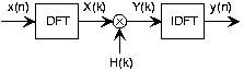
and we must compute the same length DFT of the input. To accommodate a shorter signal than DFT length, we simply zero-pad the input: Ensure that for indices extending beyond the signal's duration that the signal is zero. Frequency-domain filtering, diagrammed in Figure 1, is accomplished by storing the filter's frequency response as the DFT

, computing the input's DFT

, multiplying them to create the output's DFT

, and computing the inverse DFT of the result to yield

.
Before detailing this procedure, let's clarify why so many new issues arose in trying to develop a frequency-domain implementation of linear filtering. The frequency-domain relationship between a filter's input and output is always true:

. The Fourier transforms in this result are discrete-time Fourier transforms; for example,

. Unfortunately, using this relationship to perform filtering is restricted to the situation when we have analytic formulas for the frequency response and the input signal. The reason why we had to "invent" the discrete Fourier transform (DFT) has the same origin: The spectrum resulting from the discrete-time Fourier transform depends on the continuous frequency variable ff. That's fine for analytic calculation, but computationally we would have to make an uncountably infinite number of computations.
Note:
Did you know that two kinds of infinities can be meaningfully defined? A countably infinite quantity means that it can be associated with a limiting process associated with integers. An uncountably infinite quantity cannot be so associated. The number of rational numbers is countably infinite (the numerator and denominator correspond to locating the rational by row and column; the total number so-located can be counted, voila!); the number of irrational numbers is uncountably infinite. Guess which is "bigger?"
The DFT computes the Fourier transform at a finite set of frequencies — samples the true spectrum — which can lead to aliasing in the time-domain unless we sample sufficiently fast. The sampling interval here is

for a length-

DFT: faster sampling to avoid aliasing thus requires a longer transform calculation. Since the longest signal among the input, unit-sample response and output is the output, it is that signal's duration that determines the transform length. We simply extend the other two signals with zeros (zero-pad) to compute their DFTs.
Suppose we want to average daily stock prices taken over last year to yield a running weekly average (average over five trading sessions). The filter we want is a length-5 averager (as shown in the unit-sample response), and the input's duration is 253 (365 calendar days minus weekend days and holidays). The output duration will be

, and this determines the transform length we need to use. Because we want to use the FFT, we are restricted to power-of-two transform lengths. We need to choose any FFT length that exceeds the required DFT length. As it turns out, 256 is a power of two (

), and this length just undershoots our required length. To use frequency domain techniques, we must use length-512 fast Fourier transforms.
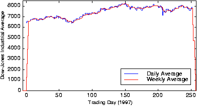
Figure 2 shows the input and the filtered output. The MATLAB programs that compute the filtered output in the time and frequency domains are
Time Domain h = [1 1 1 1 1]/5;y = filter(h,1,[djia zeros(1,4)]);Frequency Domain h = [1 1 1 1 1]/5;DJIA = fft(djia, 512);H = fft(h, 512);Y = H.*X;y = ifft(Y);Note:
The filter program has the feature that the length of its output equals the length of its input. To force it to produce a signal having the proper length, the program zero-pads the input appropriately.
MATLAB's fft function automatically zero-pads its input if the specified transform length (its second argument) exceeds the signal's length. The frequency domain result will have a small imaginary component — largest value is

— because of the inherent finite precision nature of computer arithmetic. Because of the unfortunate misfit between signal lengths and favored FFT lengths, the number of arithmetic operations in the time-domain implementation is far less than those required by the frequency domain version: 514 versus 62,271. If the input signal had been one sample shorter, the frequency-domain computations would have been more than a factor of two less (28,696), but far more than in the time-domain implementation.
An interesting signal processing aspect of this example is demonstrated at the beginning and end of the output. The ramping up and down that occurs can be traced to assuming the input is zero before it begins and after it ends. The filter "sees" these initial and final values as the difference equation passes over the input. These artifacts can be handled in two ways: we can just ignore the edge effects or the data from previous and succeeding years' last and first week, respectively, can be placed at the ends.
This textbook is open source. Download for free at http://cnx.org/contents/778e36af-4c21-4ef7-9c02-dae860eb7d14@9.72.
Explore CircuitBread


Get the latest tools and tutorials, fresh from the toaster.


