Wireline Channels

Wireline channels were the first used for electrical communications in the mid-nineteenth century for the telegraph. Here, the channel is one of several wires connecting transmitter to receiver. The transmitter simply creates a voltage related to the message signal and applies it to the wire(s). We must have a circuit—a closed path—that supports current flow. In the case of single-wire communications, the earth is used as the current's return path. In fact, the term ground for the reference node in circuits originated in single-wire telegraphs. You can imagine that the earth's electrical characteristics are highly variable, and they are. Single-wire metallic channels cannot support high-quality signal transmission having a bandwidth beyond a few hundred Hertz over any appreciable distance.

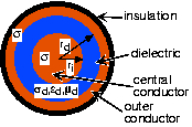
Consequently, most wireline channels today essentially consist of pairs of conducting wires (Figure 1), and the transmitter applies a message-related voltage across the pair. How these pairs of wires are physically configured greatly affects their transmission characteristics. One example is twisted pair, wherein the wires are wrapped about each other. Telephone cables are one example of a twisted pair channel. Another is coaxial cable, where a concentric conductor surrounds a central wire with a dielectric material in between. Coaxial cable, fondly called "co-ax" by engineers, is what Ethernet uses as its channel. In either case, wireline channels form a dedicated circuit between transmitter and receiver. As we shall find subsequently, several transmissions can share the circuit by amplitude modulation techniques; commercial cable TV is an example. These information-carrying circuits are designed so that interference from nearby electromagnetic sources is minimized. Thus, by the time signals arrive at the receiver, they are relatively interference- and noise-free.

Both twisted pair and co-ax are examples of transmission lines, which all have the circuit model shown in Figure 2 for an infinitesimally small length. This circuit model arises from solving Maxwell's equations for the particular transmission line geometry.

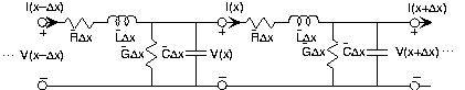
The series resistance comes from the conductor used in the wires and from the conductor's geometry. The inductance and the capacitance derive from transmission line geometry, and the parallel conductance from the medium between the wire pair. Note that all the circuit elements have values expressed by the product of a constant times a length; this notation represents that element values here have per-unit-length units. For example, the series resistance

has units of ohms/meter. For coaxial cable, the element values depend on the inner conductor's radius

, the outer radius of the dielectric

, the conductivity of the conductors

, and the conductivity

, dielectric constant

, and magnetic permittivity

of the dielectric as

For twisted pair, having a separation dd between the conductors that have conductivity σσ and common radius rr and that are immersed in a medium having dielectric and magnetic properties, the element values are then

The voltage between the two conductors and the current flowing through them will depend on distance xx along the transmission line as well as time. We express this dependence as v(x,t)v x t and i(x,t)i x t. When we place a sinusoidal source at one end of the transmission line, these voltages and currents will also be sinusoidal because the transmission line model consists of linear circuit elements. As is customary in analyzing linear circuits, we express voltages and currents as the real part of complex exponential signals, and write circuit variables as a complex amplitude—here dependent on distance—times a complex exponential:

and

. Using the transmission line circuit model, we find from KCL, KVL, and v-i relations the equations governing the complex amplitudes.

Rearranging and taking the limit

yields the so-called transmission line equations.

By combining these equations, we can obtain a single equation that governs how the voltage's or the current's complex amplitude changes with position along the transmission line. Taking the derivative of the second equation and plugging the first equation into the result yields the equation governing the voltage.

This equation's solution is

Calculating its second derivative and comparing the result with our equation for the voltage can check this solution.

Our solution works so long as the quantity

satisfies

Thus,

depends on frequency, and we express it in terms of real and imaginary parts as indicated. The quantities

and

are constants determined by the source and physical considerations. For example, let the spatial origin be the middle of the transmission line model (Figure 1). Because the circuit model contains simple circuit elements, physically possible solutions for voltage amplitude cannot increase with distance along the transmission line. Expressing γγ in terms of its real and imaginary parts in our solution shows that such increases are a (mathematical) possibility.

The voltage cannot increase without limit; because

is always positive, we must segregate the solution for negative and positive

. The first term will increase exponentially for

unless

in this region; a similar result applies to

for .

These physical constraints give us a cleaner solution.

This solution suggests that voltages (and currents too) will decrease exponentially along a transmission line. The space constant, also known as the attenuation constant, is the distance over which the voltage decreases by a factor of

. It equals the reciprocal of

, which depends on frequency, and is expressed by manufacturers in units of dB/m.

The presence of the imaginary part of

,

, also provides insight into how transmission lines work. Because the solution for

is proportional to

, we know that the voltage's complex amplitude will vary sinusoidally in space. The complete solution for the voltage has the form

The complex exponential portion has the form of a propagating wave. If we could take a snapshot of the voltage (take its picture at

), we would see a sinusoidally varying waveform along the transmission line. One period of this variation, known as the wavelength, equals

. If we were to take a second picture at some later time

, we would also see a sinusoidal voltage. Because

the second waveform appears to be the first one, but delayed—shifted to the right—in space. Thus, the voltage appeared to move to the right with a speed equal to

(assuming

). We denote this propagation speed by cc, and it equals

In the high-frequency region where

and

, the quantity under the radical simplifies to

, and we find the propagation speed to be

For typical coaxial cable, this propagation speed is a fraction (one-third to two-thirds) of the speed of light.

By using the second of the transmission line equation

, we can solve for the current's complex amplitude. Considering the spatial region

, for example, we find that

which means that the ratio of voltage and current complex amplitudes does not depend on distance.

The quantity

is known as the transmission line's characteristic impedance. Note that when the signal frequency is sufficiently high, the characteristic impedance is real, which means the transmission line appears resistive in this high-frequency regime.

Typical values for characteristic impedance are 50 and 75 Ω.

A related transmission line is the optic fiber. Here, the electromagnetic field is light, and it propagates down a cylinder of glass. In this situation, we don't have two conductors—in fact we have none—and the energy is propagating in what corresponds to the dielectric material of the coaxial cable. Optic fiber communication has exactly the same properties as other transmission lines: Signal strength decays exponentially according to the fiber's space constant and propagates at some speed less than light would in free space. From the encompassing view of Maxwell's equations, the only difference is the electromagnetic signal's frequency. Because no electric conductors are present and the fiber is protected by an opaque “insulator,” optic fiber transmission is interference-free.

To summarize, we use transmission lines for high-frequency wireline signal communication. In wireline communication, we have a direct, physical connection—a circuit—between transmitter and receiver. When we select the transmission line characteristics and the transmission frequency so that we operate in the high-frequency regime, signals are not filtered as they propagate along the transmission line: The characteristic impedance is real-valued—the transmission line's equivalent impedance is a resistor—and all the signal's components at various frequencies propagate at the same speed. Transmitted signal amplitude does decay exponentially along the transmission line. Note that in the high-frequency regime the space constant is approximately zero, which means the attenuation is quite small.