Trigonometry Fundamentals for Electromagnetic Theory

Electromagnetism calculations require a certain degree of proficiency in mathematics. Vector operations utilize trigonometry concepts, and evaluating integrals can sometimes get tedious and require a brief review of integration methods. This tutorial is a quick refresher on the mathematical concepts relevant to electromagnetic calculations, particularly trigonometry, and calculus. We will solve vector and electric field problems and give a more focused view of the mathematics involved.

Right triangles are triangles with two sides perpendicular to each other, making a right angle

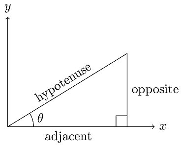
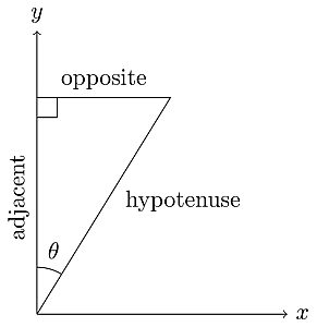
Generally, in trigonometry and our calculations, the angle of interest will be any of the other two angles. Depending on the angle of interest, the three sides of a right triangle are referred to as opposite, adjacent, and hypotenuse. The longest side is called the hypotenuse. Angles are conventionally measured counterclockwise from the positive x-axis; hence the adjacent side is usually along the x-axis, and the opposite side is usually parallel to the y-axis, as shown in Figure 1 (a). However, it is more useful to note that the adjacent side is the side that makes the angle with the hypotenuse, and the opposite side is the side opposite the angle.

(a)	(b)

Figure 1: An angle measured from (a) the x-axis and (b) the y-axis

An angle is in standard position if its vertex is located at the origin and its initial side extends along the positive x-axis. Figure 2 shows angles in standard position.

Angles in the standard position are measured from the positive x-axis, either positive (counterclockwise) or negative (clockwise).

Sine, cosine, and tangent are the main trigonometric functions that relate the angles and sides of right triangles. Sine is the ratio of the opposite side to the hypotenuse, cosine is the ratio of the adjacent side to the hypotenuse, and tangent is the ratio of the opposite side to the adjacent side. They are often written as where is an angle in radians or degrees.

The trigonometric ratios are

For angles in standard position in coordinate systems (e.g., the Cartesian or Polar coordinate systems), the signs of the trigonometric functions are determined by the position of the terminal side of the angle, that is, in what quadrant the terminal side of the angle lies. Figure 3(a) describes the signs of the functions in the four quadrants.

Figure 3: (a) Signs of trig functions in different quadrants, (b) standard angles in degrees and radians, and (c) the unit circle with trig values of standard angles

Figure 3(b): Since the unit circle has a radius of 1 unit (hence the hypotenuse is equal to 1), the coordinates where the terminal side of an angle intersects the unit circle give the (cos, sin) values of the angle. For example,

Along with these three functions are the reciprocal trigonometric functions:

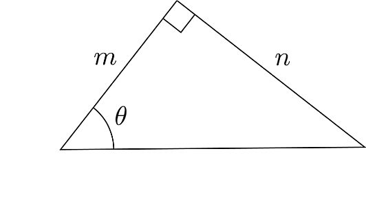
Example: What are the trigonometric ratios for the of a triangle in Fig. 4(a) and in the standard position in Fig. 4(b)?

(a)	(b)

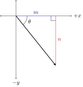
Figure 4: (a) A right triangle with an angle of interest and (b) angle with terminal side in the fourth quadrant

Solution

In the triangle in Figure 4(a), we get the hypotenuse c in terms of m and n from the Pythagorean theorem:

The three trigonometric ratios are

In Figure 4(b), the angle is in the standard position, and the terminal side is in the fourth quadrant. Hence the signs of the trigonometric functions will apply. Since the y-component is negative in the fourth quadrant, the sine is negative, and consequently, the tangent is also negative.

Therefore, the trigonometric ratios are

Trigonometric identities are equalities that hold true only for a right triangle. They are useful in solving mathematical expressions involving trigonometric functions and are based on the six trigonometric ratios. Numerous trigonometric identities are used to solve many trigonometric problems. Using these identities as formulas, complex trigonometric questions can be solved quickly. The Pythagorean Identities are fundamental trigonometric identities.

Consider the right triangle below:

An equation relating the three sides of the triangle is the Pythagorean theorem:

Dividing (1) by c², we get

By definition,

Therefore, (2) becomes

Dividing (1) by a², we get

By definition,

Therefore, (4) becomes

Dividing (1) by b², we get

By definition,

Therefore, (6) becomes

From the Pythagorean theorem (1), we derived the Pythagorean Identities:

The Pythagorean Identities can be rearranged in different ways (as in Table 2) and are ubiquitous in their utility in calculations involving trigonometric expressions.

If we are solving for an angle and the trigonometric ratio is given or known, the inverse trig function can find the angle. Inverse trig functions perform the inverse operation of normal trig functions—they find the angle with the corresponding trig ratio.

Given the trig ratio, we can isolate and solve for using the inverse trig function:

The expression is not the same as [which is equal to (x)]. In this case, -1 is not treated as an exponent but rather as a notation for the inverse of a function. Raising a number to a negative exponent gives the reciprocal or multiplicative inverse of the number. However, (x) is a function and not a quantity. The inverse of a function f is simply denoted by f^-1.

Interpretation

The inverse cosine gives us an angle with a cosine value x, that is,

To solve for we write

For example,

If we look for an angle with a cosine of ½ in Figure 3(b) and 3(c), we find two possible values for

To choose which angle is the unique solution, we look at the restricted domain of trig functions.

Recall that the domain of a function is the set of all possible inputs for the function, and the range of a function is the set of all the output values of a function.

A one-to-one function is a special function that maps every range element to exactly one unique element of its domain. In the example the output ½ maps two possible values. This means that is not a one-to-one function. This is also the case for sine and tangent. Moreover, inverse functions are only defined for one-to-one functions, i.e., a function has an inverse if and only if it is one-to-one.

Let f be a one-to-one function and f^-1 its inverse. The domain of f is the range of f^-1, and the range of f is the domain of f^-1.

Because the sine, cosine, and tangent functions are not one-to-one, they technically do not have inverse functions. Strictly speaking, the inverse sine, cosine, and tangent functions refer to the inverse of the corresponding trig functions with restricted domains. The trig functions are periodic functions, and the restricted domains make sure that every element in the range will only map one element in the domain. The domain of the trig functions is restricted as follows:

For sine, the domain is restricted to

• the range is still [-1, 1]

For cosine, the domain is restricted to

• the range is still [-1, 1]

For tangent, the domain is restricted to

• the range is still

Table 1. Domain and range of trig and inverse trig functions

Function	Domain (x)	Range (y)

From the restricted cosine domain,

If we want to find the angle we can refer to Figure 3 to find the angle where From the restricted sine domain,

We can use trigonometry to express vectors in terms of components and simplify calculations. For two-dimensional motion, we can separate the horizontal and vertical components of a vector in Figure using the following relationships for a right triangle:

Hence,

where r is the magnitude of

• is the length of the projection of on the x-axis
  
• is the length of the projection of on the y-axis

Hence, we can write as a sum of two vectors and where and

Example: Express the force vector in terms of x and y components

Solution

Since we are dealing with vectors, we take into account the direction or signs of the components.

Convention:

• and components pointing to the right and up, respectively have a positive sign
• and components pointing to the left and down, respectively have a negative sign

In the right triangle, where

Therefore,

And the vector as a sum of its components is

We can also write to indicate that the x-component points to the direction of the negative x-axis.

We can also show the other way around that from the components:

In integral calculus, trig substitutions can help evaluate integrals with certain forms of radical expressions. This type of substitution is usually indicated when the integrand has a polynomial expression that allows us to use the Pythagorean identities.

Table 2. Effective substitutions for the given radical expressions because of the specified trigonometric identities; x is the variable, and a is a constant

Expression	Substitution	Identity

Before utilizing trig substitution, it will save time to ensure that the integral cannot be evaluated easily in another way. For example, although this method can technically be used on the integrals

they can each be integrated directly by formula or a simple u-substitution.

Example

Positive charge is distributed uniformly along the y-axis between y =+ a and y =- a

Find the electric field at a point P on the x-axis at a distance x from the origin.

Solution

The figure above shows the situation. We must find the electric field due to a continuous distribution of charge. Our target variable is an expression for the electric field at P as a function of x. The x-axis is a perpendicular bisector of the line charge, so we can use a symmetry argument.

The line charge has length 2a, and we divide this into infinitesimal segments of length dy. The linear charge density is

and the charge in a segment is

The distance r from a segment at height y to point P is

so the magnitude of the field at P due to the segment at height y is

The figure also shows that the components of this field are

and

where

and

Hence,

The total field at P is the sum of the fields from all segments along the line—that is, we must integrate from y = -a to y = +a. We can start with finding E_x:

Here we encounter a radical expression in the integrand that allows us to use trig substitution.

Further inspection will tell us this cannot be evaluated with a simpler method. We proceed with trig substitution. From Table 2,

Substitute

The integral becomes

Evaluating,

Now, we undo the substitution to return to the original variable,

and evaluate from

tan^-1 (a/x) is an angle u (or in the figure) where tan(u) = a/x. Considering the sides of the right triangle, the opposite side is a, the adjacent side is x, and the hypotenuse is

The sine is therefore

Simplifying,

E_x is therefore

Using symmetry, we can conclude that E_y = 0. If there is a positive charge at P, the upper half of the line charge pushes downward on it, and the lower half pushes up with equal magnitude. The upper and lower halves of the segment contribute equally to the total field at P, and the total field is purely along the x-axis

Solving for E_y ,

The integral can be evaluated by a simple u-substitution.

Going back to the original variable y with u = x² + y² and evaluating from y = ─ a to y = +a ,

Therefore, the components are

And the electric field at P a distance x from a line charge of length 2a is

In this tutorial, we revisited and reviewed trigonometry concepts. While not a complete and in-depth tutorial on trigonometry, the objective of this review is to refamiliarize us with concepts relevant in the calculations in our tutorials on electromagnetism.