Magnetic Flux Density

Magnetic flux density is a vector field which we identify using the symbol B and which has SI units of tesla (

). Before offering a formal definition, it is useful to consider the broader concept of the magnetic field.

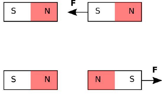
Magnetic fields are an intrinsic property of some materials, most notably permanent magnets. The basic phenomenon is probably familiar, and is shown in Figure 2.5.1. A bar magnet has “poles” identified as “N” (“north”) and “S” (“south”). The N-end of one magnet attracts the S-end of another magnet but repels the N-end of the other magnet and so on. The existence of a vector field is apparent since the observed force acts at a distance and is asserted in a specific direction. In the case of a permanent magnet, the magnetic field arises from mechanisms occurring at the scale of the atoms and electrons comprising the material. These mechanisms require some additional explanation which we shall defer for now.

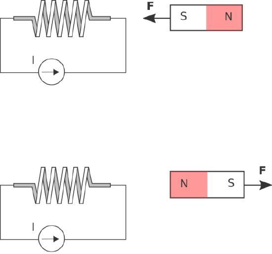
Figure 2.5.1: Evidence of a vector field from observations of the force perceived by the bar magnets on the right in the presence of the bar magnets on the left.

Magnetic fields also appear in the presence of current. For example, a coil of wire bearing a current is found to influence permanent magnets (and vice versa) in the same way that permanent magnets affect each other. This is shown in Figure 2.5.2. From this, we infer that the underlying mechanism is the same – i.e., the vector field generated by a current-bearing coil is the same phenomenon as the vector field associated with a permanent magnet. Whatever the source, we are now interested in quantifying its behavior.

Figure 2.5.2: Evidence that current can also create a magnetic field.

To begin, let us consider the effect of a magnetic field on a electrically-charged particle. First, imagine a region of free space with no electric or magnetic fields. Next, imagine that a charged particle appears. This particle will experience no force. Next, a magnetic field appears; perhaps this is due to a permanent magnet or a current in the vicinity. This situation is shown in Figure 2.5.2 (top). Still, no force is applied to the particle. In fact, nothing happens until the particle in set in motion. Figure 2.5.3 (bottom) shows an example. Suddenly, the particle perceives a force. We’ll get to the details about direction and magnitude in a moment, but the main idea is now evident. A magnetic field is something that applies a force to a charged particle in motion, distinct from (in fact, in addition to) the force associated with an electric field.

Figure 2.5.3: The force perceived by a charged particle that is (top) motionless and (bottom) moving with velocity

, which is perpendicular to the plane of this document and toward the reader.

Now, it is worth noting that a single charged particle in motion is the simplest form of current. Remember also that motion is required for the magnetic field to influence the particle. Therefore, not only is current the source of the magnetic field, the magnetic field also exerts a force on current. Summarizing:

The magnetic field describes the force exerted on permanent magnets and currents in the presence of other permanent magnets and currents.

So, how can we quantify a magnetic field? The answer from classical physics involves another experimentally-derived equation that predicts force as a function of charge, velocity, and a vector field

representing the magnetic field. Here it is: The force applied to a particle bearing charge

where

is the velocity of the particle and “

” denotes the cross product. The cross product of two vectors is in a direction perpendicular to each of the two vectors, so the force exerted by the magnetic field is perpendicular to both the direction of motion and the direction in which the magnetic field points.

The reader would be well-justified in wondering why the force exerted by the magnetic field should perpendicular to

. For that matter, why should the force depend on

? These are questions for which classical physics provides no obvious answers. Effective answers to these questions require concepts from quantum mechanics, where we find that the magnetic field is a manifestation of the fundamental and aptly-named electromagnetic force. The electromagnetic force also gives rises to the electric field, and it is only limited intuition, grounded in classical physics, that leads us to perceive the electric and magnetic fields as distinct phenomena. For our present purposes – and for most commonly-encountered engineering applications – we do not require these concepts. It is sufficient to accept this apparent strangeness as fact and proceed accordingly.

Dimensional analysis of Equation 2.5.1 reveals that

has units of (N⋅s)/(C⋅m). In SI, this combination of units is known as the tesla (

We refer to

as magnetic flux density, and therefore tesla is a unit of magnetic flux density. A fair question to ask at this point is: What makes this a flux density? The short answer is that this terminology is somewhat arbitrary, and in fact is not even uniformly accepted. In engineering electromagnetics, the preference for referring to

as a “flux density” is because we frequently find ourselves integrating

over a mathematical surface. Any quantity that is obtained by integration over a surface is referred to as “flux,” and so it becomes natural to think of

as a flux density; i.e., as flux per unit area. The SI unit for magnetic flux is the weber (

). Therefore,

may alternatively be described as having units of

/m², and 1

/m² = 1

Magnetic flux density (

, T or

/m²) is a description of the magnetic field that can be defined as the solution to Equation 2.5.1.

Figure 2.5.4: The magnetic field of a bar magnet, illustrating field lines.

When describing magnetic fields, we occasionally refer to the concept of a field line, defined as follows:

A magnetic field line is the curve in space traced out by following the direction in which the magnetic field vector points. This concept is illustrated in Figure 2.5.4 for a permanent bar magnet and Figure 2.5.5 for a current-bearing coil.

Figure 2.5.5: The magnetic field of a current-bearing coil, illustrating field lines.

Magnetic field lines are remarkable for the following reason:

A magnetic field line always forms a closed loop.

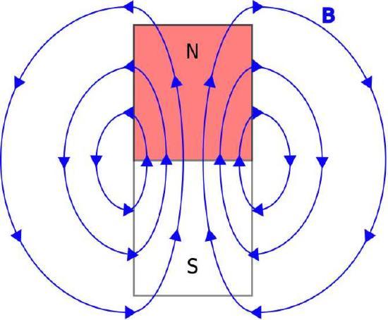
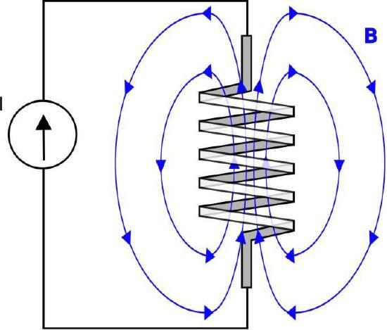
This is true in a sense even for field lines which seem to form straight lines (for example, those along the axis of the bar magnet and the coil in Figures 2.5.4 and 2.5.5, since a field line that travels to infinity in one direction reemerges from infinity in the opposite direction.