- Electromagnetics I
- Ch 3
- Loc 3.13
Standing Waves
A standing wave consists of waves moving in opposite directions. These waves add to make a distinct magnitude variation as a function of distance that does not vary in time.
To see how this can happen, first consider that an incident wave

, which is traveling in the

axis along a lossless transmission line. Associated with this wave is a reflected wave

, where

is the voltage reflection coefficient. These waves add to make the total potential

The magnitude of

is most easily found by first finding

, which is:

Let

be the phase of
; i.e.,

Then, continuing from the previous expression:

The quantity in square brackets can be reduced to a cosine function using the identity

yielding:

Recall that this is

.

is therefore the square root of the above expression:

Thus, we have found that the magnitude of the resulting total potential varies sinusoidally along the line. This is referred to as a standing wave because the variation of the magnitude of the phasor resulting from the interference between the incident and reflected waves does not vary with time.
We may perform a similar analysis of the current, leading to:

Again we find the result is a standing wave.
Now let us consider the outcome for a few special cases.
Matched load. When the impedance of the termination of the transmission line,

, is equal to the characteristic impedance of the transmission line,

,

and there is no reflection. In this case, the above expressions reduce to

and

, as expected.
Open or Short-Circuit. In this case,

and we find:


where

for an open circuit and

for a short circuit. The result for an open circuit termination is shown in Figure 3.13.1 (a) (potential) and (b) (current). The result for a short circuit termination is identical except the roles of potential and current are reversed. In either case, note that voltage maxima correspond to current minima, and vice versa.
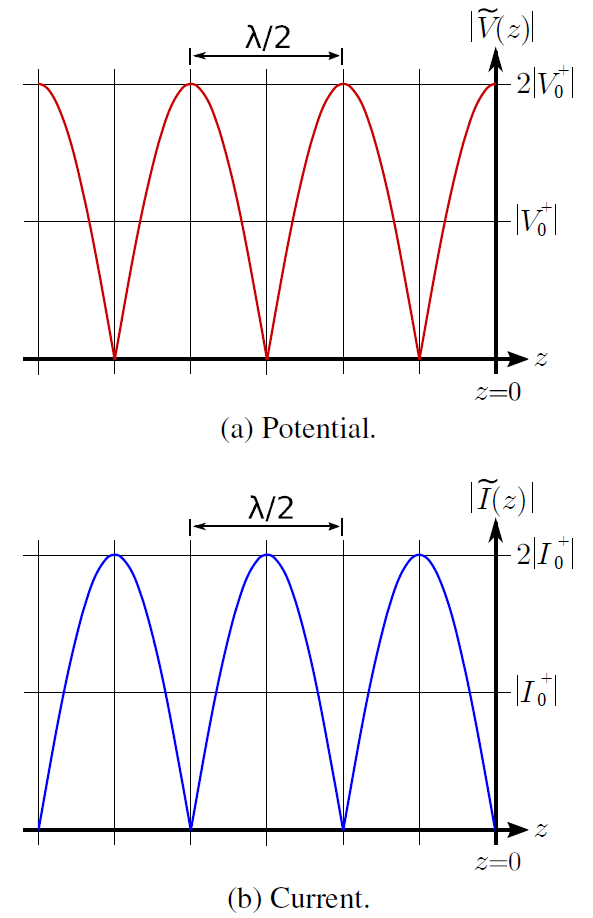
Also note:
The period of the standing wave is

; i.e., one-half of a wavelength.
This can be confirmed as follows. First, note that the frequency argument of the cosine function of the standing wave is

. This can be rewritten as

, so the frequency of variation is

and the period of the variation is

. Since

, we see that the period of the variation is
. Furthermore, this is true regardless of the value of
.
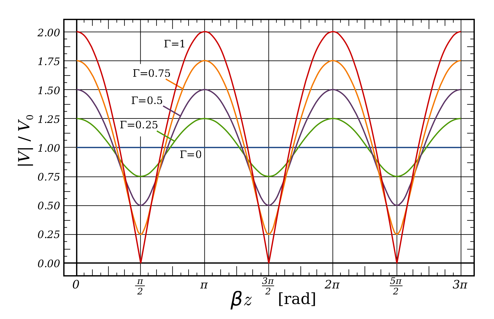
Mismatched loads
A common situation is that the termination is neither perfectly-matched (
) nor an open/short circuit (

). Examples of the resulting standing waves are shown in Figure 3.13.2.
Additional Reading
- “Standing Wave” on Wikipedia
Ellingson, Steven W. (2018) Electromagnetics, Vol. 1. Blacksburg, VA: VT Publishing. https://doi.org/10.21061/electromagnetics-vol-1 CC BY-SA 4.0
Explore CircuitBread


Get the latest tools and tutorials, fresh from the toaster.


