Telegrapher’s Equations

In this section, we derive the equations that govern the potential

and current

along a transmission line that is oriented along the

$z$

axis. For this, we will employ the lumped-element model developed in Section 3.4.

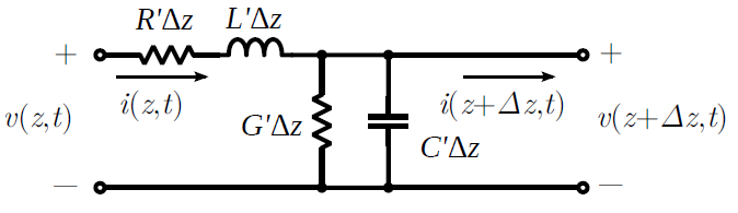
Figure 3.5.1: Lumped-element equivalent circuit transmission line model, annotated with sign conventions for potentials and currents.

To begin, we define voltages and currents as shown in Figure 3.5.1. We assign the variables

and

to represent the potential and current on the left side of the segment, with reference polarity and direction as shown in the figure. Similarly we assign the variables

and

to represent the potential and current on the right side of the segment, again with reference polarity and direction as shown in the figure. Applying Kirchoff’s voltage law from the left port, through

and

, and returning via the right port, we obtain:

Moving terms referring to current to the right side of the equation and then dividing through by

, we obtain

Then taking the limit as

Applying Kirchoff’s current law at the right port, we obtain:

Moving terms referring to potential to the right side of the equation and then dividing through by

, we obtain

Taking the limit as

Equations 3.5.3 and 3.5.6 are the telegrapher’s equations. These coupled (simultaneous) differential equations can be solved for

and

given

and suitable boundary conditions.

The time-domain telegrapher’s equations are usually more than we need or want. If we are only interested in the response to a sinusoidal stimulus, then considerable simplification is possible using phasor representation.¹ First we define phasors

and

through the usual relationship:

Now we see:

In other words,

expressed in phasor representation is simply

; and

In other words,

expressed in phasor representation is

. Therefore, Equation 3.5.3 expressed in phasor representation is:

Following the same procedure, Equation 3.5.6 expressed in phasor representation is found to be:

Equations 3.5.9 and 3.5.10 are the telegrapher’s equations in phasor representation.

The principal advantage of these equations over the time-domain versions is that we no longer need to contend with derivatives with respect to time – only derivatives with respect to distance remain. This considerably simplifies the equations.