Time Response Analysis and Standard Test Signals | Control Systems 2.1

In the previous tutorial, we learnt about signal flow graphs and completed the first chapter in our control systems tutorial series. With this tutorial, we shall be starting with the Time Response analysis of control systems.

Time response analysis is nothing but the analysis of performance of the system in the time domain. In other words, it’s knowing how different system variables change their state with respect to time. This is required for us to control the speed of the response, minimize the error and a lot of other things that we’ll learn as we go ahead with this chapter.

All systems have some energy storing elements like inductors, capacitors, flywheels, etc. and they cannot be avoided. When a certain input is given, the output doesn’t change instantly as these elements can’t change the energy they store instantly as they need a certain amount of time to change the amount of energy the store. The time that is required for the system to go from one state to another state is what we call transient time and the response of the system during this time is called the transient response. If a system is stable and well-designed, the system will settle close to the desired output and this response after the system settles is the steady state response.

Let’s take a simple example here,

When we kick a ball in a set up as shown above, the ball bounces a few times due to its kinetic energy and then settles. The response when the ball is still bouncing is the transient response and once it settles, it’s the steady state.

Another way to look at the time response is by analyzing how the system responds to the stored energy of the system with no input given which is called the natural response of the system. Then how the system responds to a given input but with no energy stored initially in the system is called the forced response.

An example for this could be a series RLC circuit. Natural response would be the response of the circuit to the initial inductor currents and capacitor voltages with all independent voltage and current sources set to zero. And the forced response would be the response of the circuit only to the external sources while the initial conditions are zero.

However, the complete response of the system is given by the combination of both responses i.e., transient and steady state responses or natural and forced responses.

In this tutorial series we shall stick to the former one (transient and steady state responses) as it is more popular as well as convenient.

Let’s speak more mathematically now and formally define the transient and steady state responses.

Transient Response [y_tr(t)]

It is that part of the time response that goes to zero as time tends to infinite (ideally). Transient response can be associated to anything that affects the equilibrium of a system like switching, change in input, noise, etc.

Mathematically,

Steady State Response [y_ss(t)]

Steady state response is the response of a system after transient practically disappears as time goes to infinity (ideally).

The complete response [y(t)] of a control system is the sum of the transient and steady state response.

Generally, control systems are required to perform both under transient as well as steady state conditions and having feedback enables us to control both of these responses. With the knowledge of the transfer function of the system, we can find the expression for the response of the system for a specific input by taking the inverse of the laplace transform which we have discussed earlier.

To know the response, we would need two things. First is the transfer function of the system which we already know how to obtain. Second is the input. Simple isn’t it? But here’s the problem. The input is not fully known ahead of time as inputs can be random in nature and can be situation dependent. This makes it almost impossible to represent the myriad of possible inputs mathematically. As a solution to this, the performance of a control system can be judged based on its response to a few common inputs such as a sudden shock, a sudden change in its state, an input that linearly increases with time, and an input that increases quadratically. These are called the standard test signals.

In signals perspective, these are - an impulse, a step, a ramp, and a parabolic signal.

Now, let’s understand these signals one by one.

1. The Step Signal.

Consider the circuit below.

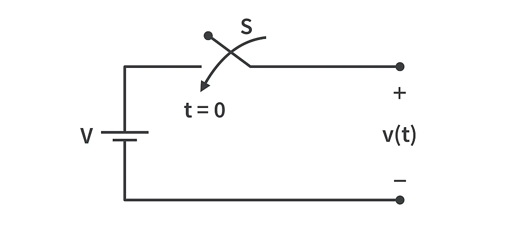
Let the switch be closed at time t = 0.

Now,

Before the switch is closed,

After the switch is closed,

Graphically, this looks like the following.

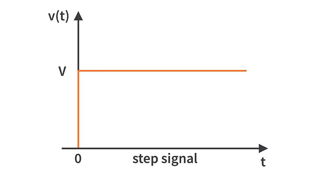
This is a step signal and more often used is the unit step signal which is denoted by u(t) and is defined as

The Laplace transform of the step signal will be

The step signal represents the sudden application of an input to the system.

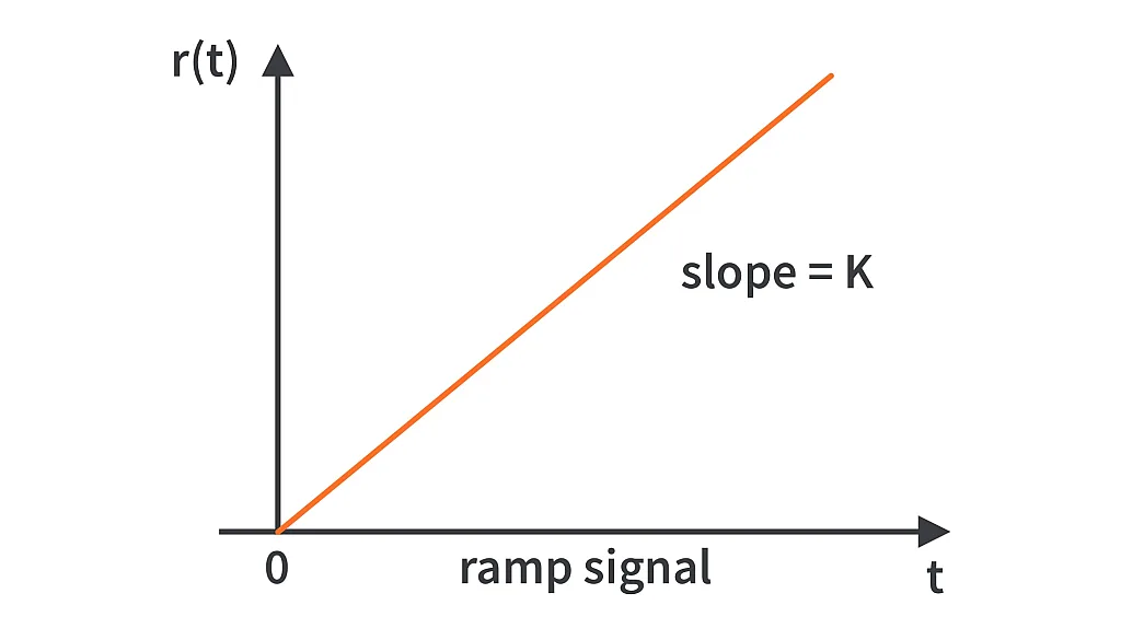
2) The Ramp Signal.

A ramp signal starts from the origin and rises linearly with time with a slope K.

Mathematically,

Let r(t) be the ramp signal,

then

Where K is the slope.

Graphically,

The Laplace transform of the ramp signal will be

With K = 1 for the unit ramp signal.

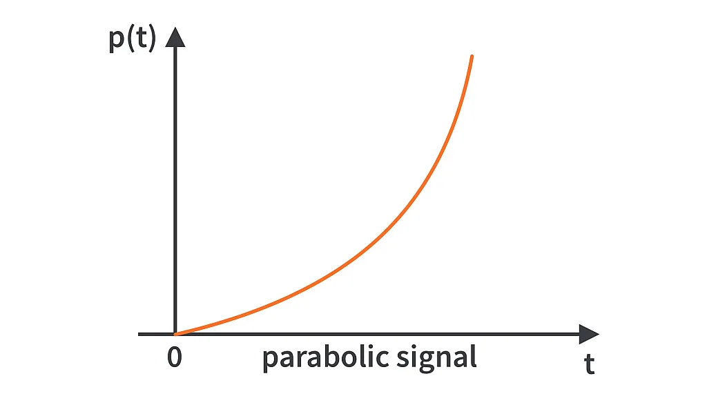
3) The Parabolic Signal.

The parabolic signal starts from zero and is a quadratic function of time.

Mathematically,

Let p(t) be the parabolic signal,

then

Graphically,

The Laplace transform of the parabolic signal will be

And K = 1 for the unit parabolic signal.

4) The Impulse Signal.

An impulse signal [δ(t)] is a tall and narrow signal which is obtained as shown.

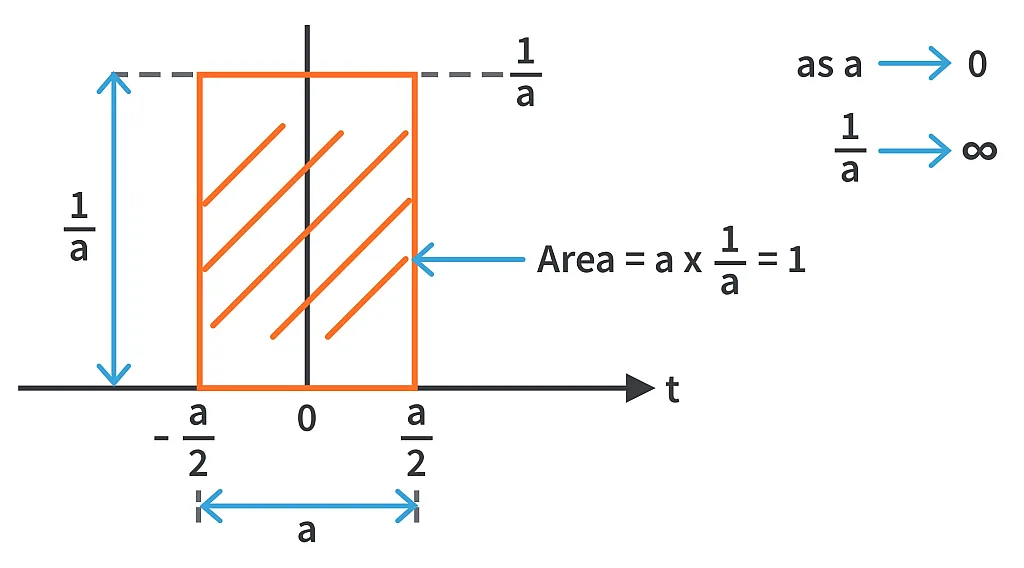
As a becomes very small (almost zero), 1/a becomes infinitely tall. This means that the width of the above shown rectangle becomes essentially 0 and the height becomes infinite yet their area remains equal to 1.

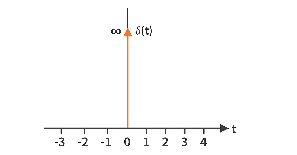
Hence the impulse signal or the impulse function takes zero value for all values of time except for t = 0.

As the area remains equal to 1, we can define the impulse signal mathematically as

and

The Laplace transform of the impulse signal will be

The impulse signal represents a sudden shock to the system.

By analyzing the response of the system to these four test signals, we should be able to judge the performance of most of the systems. Hence, we can say that these signals are the four pillars in the time response analysis. To analyze the transient response of the system, it is sufficient to test with any one of these signals as the transient response is independent of the input and depends on the nature of the system transfer function. This will gain more clarity as we proceed further. The step signal is used more frequently to analyze the transient response.

To summarize, we learnt what time response means and what it actually comprises. Then we understood the need for standard test signals and learnt about these test signals in detail.

In the next tutorial, we shall start with the time response analysis of first order systems applying the learnt test signals. Until then, try applying these test signals on random systems (like giving a quick kick to a football or a quick bang on a bell mimicking an impulse) and see how they respond.