Vector Arithmetic
A vector is a mathematical object that has both a scalar part (i.e., a magnitude and possibly a phase), as well as a direction. Many physical quantities are best described as vectors. For example, the rate of movement through space can be described as speed; i.e., as a scalar having SI base units of m/s. However, this quantity is more completely described as velocity; i.e., as a vector whose scalar part is speed and direction indicates the direction of movement. Similarly, force is a vector whose scalar part indicates magnitude (SI base units of N), and direction indicates the direction in which the force is applied. Electric and magnetic fields are also best described as vectors.
In mathematical notation, a real-valued vector

is said to have a magnitude

and direction

such that

where
is a unit vector (i.e., a real-valued vector having magnitude equal to one) having the same direction as
. If a vector is complex-valued, then

is similarly complex-valued.
Cartesian Coordinate System
Fundamentals of vector arithmetic are most easily grasped using the Cartesian coordinate system. This system is shown in Figure 4.1.1. Note carefully the relative orientation of the

,

, and

axes. This orientation is important. For example, there are two directions that are perpendicular to the

plane (in which the
- and
-axes lie), but the

axis is specified to be one of these in particular.

Position-Fixed vs. Position-Free Vectors
It is often convenient to describe a position in space as a vector for which the magnitude is the distance from the origin of the coordinate system and for which the direction is measured from the origin toward the position of interest. This is shown in Figure 4.1.2. These position vectors are “position-fixed” in the sense that they are defined with respect to a single point in space, which in this case is the origin. Position vectors can also be defined as vectors that are defined with respect to some other point in space, in which case they are considered position-fixed to that position.

Figure 4.1.2: Position vectors. The vectors

and

are position-fixed and refer to particular locations.
Position-free vectors, on the other hand, are not defined with respect to a particular point in space. An example is shown in Figure 4.1.2. Particles 1 m apart may both be traveling at 2 m/s in the same direction. In this case, the velocity of each particle can be described using the same vector, even though the particles are located at different points in space.

Figure 4.1.3: Two particles exhibiting the same velocity. In this case, the velocity vectors
and
are position-free and equal.
Position-free vectors are said to be equal if they have the same magnitudes and directions. Position-fixed vectors, on the other hand, must also be referenced to the same position (e.g., the origin) to be considered equal.
Basis Vectors
Each coordinate system is defined in terms of three basis vectors which concisely describe all possible ways to traverse three-dimensional space. A basis vector is a position-free unit vector that is perpendicular to all other basis vectors for that coordinate system. The basis vectors

,

, and

of the Cartesian coordinate system are shown in Figure 4.1.4. In this notation,
indicates the direction in which
increases most rapidly,
indicates the direction in which
increases most rapidly, and
indicates the direction in which
increases most rapidly. Alternatively, you might interpret
,
, and
as unit vectors that are parallel to the
-,
-, and
-axes and point in the direction in which values along each axis increase.

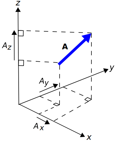
Vectors in the Cartesian Coordinate System
In Cartesian coordinates, we may describe any vector
as follows:

where

,

, and

are scalar quantities describing the components of
in each of the associated directions, as shown in Figure 4.1.5. This description makes it clear that the magnitude of
is:

and therefore, we can calculate the associated unit vector as

Vector Addition and Subtraction
It is common to add and subtract vectors. For example, vectors describing two forces
and

applied to the same point can be described as a single force vector

that is the sum of
and
; i.e.,

. This addition is quite simple in the Cartesian coordinate system:

In other words, the
component of
is the sum of the
components of
and
, and similarly for
and
. From the above example, it is clear that vector addition is commutative; i.e.,

In other words, vectors may be added in any order. Vector subtraction is defined similarly:

In other words, the
component of

is the difference of the
components of
and
, and similarly for
and
. Like scalar subtraction, vector subtraction is not commutative.
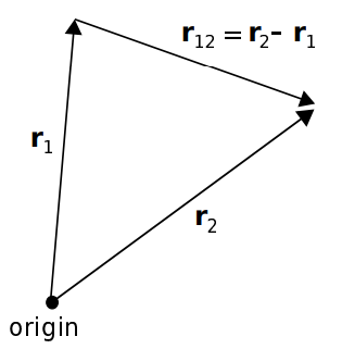
Relative Positions and Distances
A common task in vector analysis is to describe the position of one point in space relative to a different point in space. Let us identify those two points using the position vectors
and
, as indicated in Figure 4.1.6. We may identify a third vector

as the position of
relative to
:

Now

is the distance between these points, and

is a unit vector indicating the direction to
from
.
Exercise
Example 4.1.1: Direction and distance between positions
Consider two positions, identified using the position vectors

and

, both expressed in units of meters. Find the direction vector that points from
to
, the distance between these points, and the associated unit vector.
Solution:
The vector that points from
to
is

The distance between
and
is simply the magnitude of this vector:

The unit vector

is simply

normalized to have unit magnitude:

Multiplication of a Vector by a Scalar
Let’s say a particular force is specified by a vector

. What is the new vector if this force is doubled? The answer is simply

– that is, twice the magnitude applied in the same direction. This is an example of scalar multiplication of a vector. Generalizing, the product of the scalar

and the vector
is simply

.

Scalar (“Dot”) Product of Vectors
Another common task in vector analysis is to determine the similarity in the direction in which two vectors point. In particular, it is useful to have a metric which, when applied to the vectors

and

, has the following properties (Figure 4.1.7):
- If is perpendicular to , the result is zero.
- If and point in the same direction, the result is
 .
. - If and point in opposite directions, the result is
 .
. - Results intermediate to these conditions depend on the angle
 between and , measured as if and were arranged “tail-to-tail” as shown in Figure 4.1.8.

In vector analysis, this operator is known as the scalar product (not to be confused with scalar multiplication) or the dot product. The dot product is written

and is given in general by the expression:

Note that this expression yields the special cases previously identified, which are

,

, and

, respectively. The dot product is commutative; i.e.,

The dot product is also distributive; i.e.,

The dot product has some other useful properties. For example, note:

which looks pretty bad until you realize that

and any other dot product of basis vectors is zero. Thus, the whole mess simplifies to:

This is the square of the magnitude of
, so we have discovered that

Applying the same principles to the dot product of potentially different vectors
and
, we find:

This is a particularly easy way to calculate the dot product, since it eliminates the problem of determining the angle
. In fact, an easy way to calculate
given
and
is to first calculate the dot product using Equation 4.1.19 and then use the result to solve Equation 4.1.12 for
.
Exercise
Example 4.1.2: Angle between two vectors
Consider the position vectors

and

, both expressed in units of meters. Find the angle between these vectors.
From Equation 4.1.7

where

,

, and
is the angle we seek. From Equation 4.1.14:

also

so

Taking the inverse cosine, we find

.
Cross Product
The cross product is a form of vector multiplication that results in a vector that is perpendicular to both of the operands. The definition is as follows:

As shown in Figure 4.1.9, the unit vector

is determined by the “right hand rule.” Using your right hand, curl your fingers to traverse the angle

beginning at
and ending at
, and then
points in the direction of your fully-extended thumb.

Figure 4.1.9: The cross product

.
It should be apparent that the cross product is not commutative but rather is anticommutative; that is,

You can confirm this for yourself using either Equation 4.1.24 or by applying the right-hand rule.
The cross product is distributive:

There are two useful special cases of the cross product that are worth memorizing. The first is the cross product of a vector with itself, which is zero:

The second is the cross product of vectors that are perpendicular; i.e., for which

. In this case:

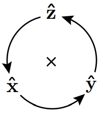
Using these principles, note:

whereas


A useful diagram that summarizes these relationships is shown in Figure 4.1.10.
It is typically awkward to “manually” determine
in Equation 4.1.24. However, in Cartesian coordinates the cross product may be calculated as:

This may be easier to remember as a matrix determinant:

Similar expressions are available for other coordinate systems.
Vector analysis routinely requires expressions involving both dot products and cross products in different combinations. Often, these expressions may be simplified, or otherwise made more convenient, using the vector identities listed in Appendix B3.
Additional Reading
- “Vector field” on Wikipedia.
- ”Vector algebra” on Wikipedia.
Ellingson, Steven W. (2018) Electromagnetics, Vol. 1. Blacksburg, VA: VT Publishing. https://doi.org/10.21061/electromagnetics-vol-1 CC BY-SA 4.0
Explore CircuitBread


Get the latest tools and tutorials, fresh from the toaster.


