The Sampling Theorem

Because of the way computers are organized, signal must be represented by a finite number of bytes. This restriction means that both the time axis and the amplitude axis must be quantized: They must each be a multiple of the integers. ¹ Quite surprisingly, the Sampling Theorem allows us to quantize the time axis without error for some signals. The signals that can be sampled without introducing error are interesting, and as described in the next section, we can make a signal "samplable" by filtering. In contrast, no one has found a way of performing the amplitude quantization step without introducing an unrecoverable error. Thus, a signal's value can no longer be any real number. Signals processed by digital computers must be discrete-valued: their values must be proportional to the integers. Consequently, analog-to-digital conversion introduces error.

Digital transmission of information and digital signal processing all require signals to first be "acquired" by a computer. One of the most amazing and useful results in electrical engineering is that signals can be converted from a function of time into a sequence of numbers without error: We can convert the numbers back into the signal with (theoretically) no error. Harold Nyquist, a Bell Laboratories engineer, first derived this result, known as the Sampling Theorem, in the 1920s. It found no real application back then. Claude Shannon, also at Bell Laboratories, revived the result once computers were made public after World War II.

The sampled version of the analog signal

is

, with

known as the sampling interval. Clearly, the value of the original signal at the sampling times is preserved; the issue is how the signal values between the samples can be reconstructed since they are lost in the sampling process. To characterize sampling, we approximate it as the product

, with

being the periodic pulse signal. The resulting signal, as shown in Figure 1, has nonzero values only during the time intervals

,

.

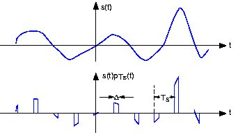
For our purposes here, we center the periodic pulse signal about the origin so that its Fourier series coefficients are real (the signal is even).

If the properties of

and the periodic pulse signal are chosen properly, we can recover

from

by filtering.

To understand how signal values between the samples can be "filled" in, we need to calculate the sampled signal's spectrum. Using the Fourier series representation of the periodic sampling signal,

Considering each term in the sum separately, we need to know the spectrum of the product of the complex exponential and the signal. Evaluating this transform directly is quite easy.

Thus, the spectrum of the sampled signal consists of weighted (by the coefficients

) and delayed versions of the signal's spectrum (Figure 2).

In general, the terms in this sum overlap each other in the frequency domain, rendering recovery of the original signal impossible. This unpleasant phenomenon is known as aliasing.

If, however, we satisfy two conditions:

• The signal is bandlimited—has power in a restricted frequency range—to Hz, and
• the sampling interval is small enough so that the individual components in the sum do not overlap— ,

aliasing will not occur. In this delightful case, we can recover the original signal by lowpass filtering

with a filter having a cutoff frequency equal to

Hz. These two conditions ensure the ability to recover a bandlimited signal from its sampled version: We thus have the Sampling Theorem.

The frequency

, known today as the Nyquist frequency and the Shannon sampling frequency, corresponds to the highest frequency at which a signal can contain energy and remain compatible with the Sampling Theorem. High-quality sampling systems ensure that no aliasing occurs by unceremoniously lowpass filtering the signal (cutoff frequency being slightly lower than the Nyquist frequency) before sampling. Such systems therefore vary the anti-aliasing filter's cutoff frequency as the sampling rate varies. Because such quality features cost money, many sound cards do not have anti-aliasing filters or, for that matter, post-sampling filters. They sample at high frequencies, 44.1 kHz for example, and hope the signal contains no frequencies above the Nyquist frequency (22.05 kHz in our example). If, however, the signal contains frequencies beyond the sound card's Nyquist frequency, the resulting aliasing can be impossible to remove.

If we satisfy the Sampling Theorem's conditions, the signal will change only slightly during each pulse. As we narrow the pulse, making

smaller and smaller, the nonzero values of the signal

will simply be

, the signal's samples. If indeed the Nyquist frequency equals the signal's highest frequency, at least two samples will occur within the period of the signal's highest frequency sinusoid. In these ways, the sampling signal captures the sampled signal's temporal variations in a way that leaves all the original signal's structure intact.

• 1

  We assume that we do not use floating-point A/D converters.