Time Response Specifications | Control Systems 2.4
Published
In the previous tutorial, we learned about second order systems and we saw how they responded to impulse and step inputs. We also pointed out that control systems are usually designed to be underdamped. If we consider higher order systems, they usually have two poles which are underdamped and dominate the other poles. Hence, even the higher order systems are generally underdamped in nature. Now, coming to this tutorial, we shall learn about time response specifications.
Let’s consider the following questions:
- How fast does the system move to follow the input?
- How much oscillation is in the response of the system?
- How long does it take to reach the final value, from a practical standpoint?
The specifications which answer the above questions are called the time response specifications. In other words, these are the specifications which quantify the response of a system. These are specified as a part of the design requirements of a control system.
These specifications generally refer to the performance indices of a step response of a system. Why only the step response? It's just because it is easier to generate a step response and can be used to generalise and compare systems based on their step responses.
Consider the step response of an underdamped system as shown below.
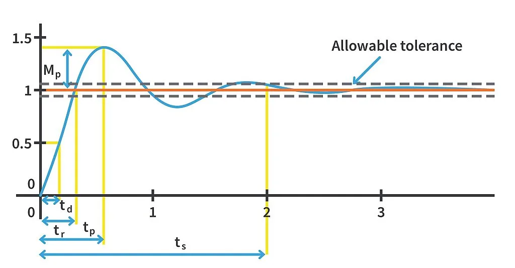
We shall now define certain common time response specifications.
1. Delay time (td) – It is the time required for the response to reach 50% of the final value in the first instance.
2. Rise time (tr) – It is the time required for the response to rise from 10% to 90% of the final value for overdamped systems and from 0 to 100% of the final value in the case of underdamped systems, in the first instance.
3. Peak time (tp) – It is the time required for the response to reach the peak value of the time response.
4. Peak overshoot (Mp) – It is the normalised difference between the peak value of the time response and the steady state value.

5. Settling time (ts) – Time required for the response to reach and stay within a specified tolerance band of its final value or steady state value. This tolerance band is usually 2% to 5%.
It is worth noting that peak time and peak overshoot are not defined for overdamped and critically damped systems. This makes sense as there will not be any peak in these systems.
Consider a second order system

As an example, take


Hence the system is

We’ll now bring back the equation that we derived for the step response of underdamped second order system

Expression for delay time
The expression for the delay time is derived empirically and is as shown below.

If we consider the chosen system,

Expression for rise time
As discussed earlier, the rise time is the time taken by the step response to go from 0 to 100% of the final value that is 1.

For this expression to come true,


For the example that we have considered,

Expression for peak time
At the peak, the derivative of the response is zero,

Solving this equation,

As we know that


So, the expression reduces to,


For the first peak,


For our example,

Expression for peak overshoot
The overshoot corresponding to the


For example,

Expression for settling time
As discussed earlier, the time required for the response to reach and stay within a specified tolerance band of its final value or steady state value.

For our example, we shall consider a 2% tolerance band.

Now, we shall deduce certain observations from these expressions.
Consider two poles of an underdamped second order system as shown,
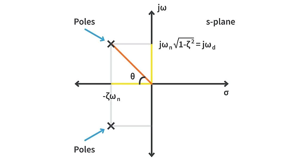
The imaginary part of the poles is inversely proportional to the peak time tp and the real part of the poles is inversely proportional to the settling time ts. Also, if you look at the expression for peak overshoot Mp, for it to remain same, the ratio

should remain constant. Hence, the real and imaginary parts of the poles would have to move proportionately.
Therefore, you can play with the poles of the system to adjust the parameters as per the design requirements.
The illustrations below will make it clear.
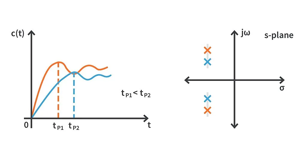
As we can observe, the imaginary part of the poles colored green is less than that of red and thus, its peak time is more.
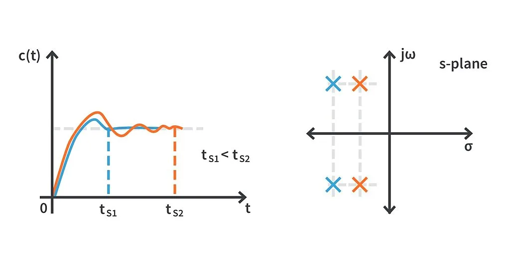
The magnitude of the real part of the poles colored green is more as compared to the poles in red. Hence, the settling time of the system represented by green poles is lesser.
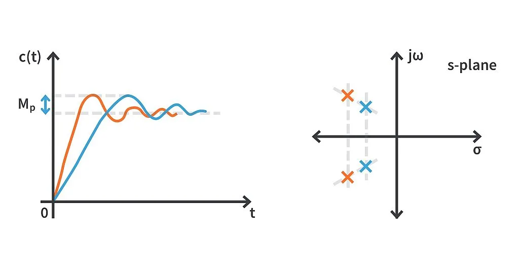
The peak overshoot is the same in both cases, but the peak time is different.
These specifications play an important role in the design and analysis of a system. The rise time, delay time, peak time, and settling time revolves around the speed of the system response and the peak overshoot gives an idea of the tolerance needed for a particular system. Designing is a reverse process of analysis so, with the specifications in hand, we can find out the damping factor and the natural frequency of the system to be designed through these specifications.
To summarize – in this tutorial, we learned about the delay time, rise time, peak time, settling time, peak overshoot, and their importance in designing a system. We also saw how these specifications relate to the location of poles of a system and how this concept can be made use of while designing a system. In the next tutorial, we shall proceed with our journey with time response analysis with the final tutorial of this chapter of error analysis.

Authored By
Kushal Gowda
An Electrical and Electronics Engineer. Loves playing Table Tennis, Cricket and Badminton . Always ready to learn and teach. His fields of interest include power electronics, e-Drives, control theory and battery systems.

Related Tutorials

Explore CircuitBread
- 244 Tutorials
- 9 Textbooks
- 12 Study Guides
- 31 Tools
- 104 EE FAQs
- 295 Equations Library
- 213 Reference Materials
- 97 Glossary of Terms
Friends of CircuitBread
-

Free Semiconductor Lifecycle Webinars
-

Relays, Switches & Connectors Knowledge Series
-

Free YouTube Product Training Guides


Get the latest tools and tutorials, fresh from the toaster.


