Second Order Systems | Control Systems 2.3

In the previous tutorial, we learned about first order systems and how they respond to various inputs with the help of Scilab and XCOS. In this tutorial we will continue our time response analysis journey with second order systems.

As you might have already guessed, second order systems are those systems where the highest power of ‘s’ in the denominator of the transfer function is two. In other words, these are systems with two poles.

Before we go ahead and look at the standard form of a second order system, it is essential for us to know a few terms:

• System damping ratio (ζ) - It is a dimensionless quantity describing the decay of oscillations during a transient response. We know the symbol looks weird and it's hard to write. You can modify it for your comfort. But verbally, it is a zeta.
• System natural frequency (ω_n) - It is the angular frequency at which system tends to oscillate in the absence of damping force. That symbol is a lower-case omega.
• System damped frequency (ω_d) - It is the angular frequency at which system tends to oscillate in the presence of damping force. Also,

Don’t worry, these terms will start making more sense when we start looking at the response of the second order system. For now, just know what they are.

With this being done, now we shall look at the standard form of a second order system.

where

• R(s) is the input,
• C(s) is the output,
• G(s) is the forward path gain, and
• H(s) is the feedback gain.

In the standard form of a second order system,

and

The response of the second order system mainly depends on its damping ratio ζ. For a particular input, the response of the second order system can be categorized and analyzed based on the damping effect caused by the value of ζ -

1. ζ > 1 :- overdamped system
2. ζ = 1 :- critically damped system
3. 0 < ζ < 1 :- underdamped system
4. ζ = 0 :- undamped system

Here we shall ignore the negative damping ratio ζ as negative damping results in oscillations with increasing amplitude resulting in unstable systems. We shall take this up later when we study the stability of control systems.

Now, if you are wondering what damping means, it is just the effect created in an oscillatory system that opposes the oscillations in that system. We just discussed the categories of systems based on its damping ratio ζ above. Now, we shall formally define them and understand what they physically mean.

• Overdamped systems - Transients in this type of system exponentially decay to steady state without any oscillations.
• Critically damped systems - Transients in this type of system decay to steady state without any oscillations in the shortest possible time.
• Underdamped systems - Transients in this type of system oscillates with the amplitude of the oscillation gradually decreasing to zero.
  
• Undamped systems - The system keeps oscillating at its natural frequency without any decay in amplitude.

The illustration below will give a better idea,

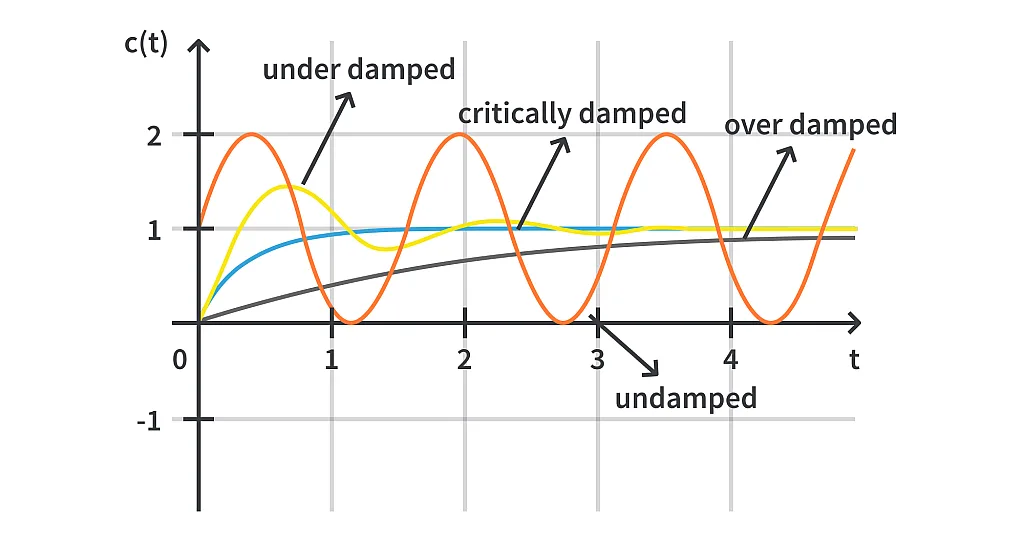
This is actually the step response of a second order system with a varied damping ratio. We shall look at this in detail in the later part of the tutorial.

With this, we shall start with the impulse response of the second order system. We will skip a few basic steps here and there. Feel free to comment below in case you didn’t follow anything.

For a unit impulse, R(s) = 1

Let the standard form of the second order system be

So,

We shall see all the cases of damping. For this let’s use Scilab.

If we substitute 0 for ζ in the equation for C(s), we get

Taking the inverse Laplace transform,

As an example, consider ω_n = 5 which gives c(t) = 5sin(5t)

Putting this in Scilab using the code below (very similar to what was used in the previous tutorial).

And what we obtain is,

which justifies what we obtained theoretically.

Next,

We know,

Taking inverse Laplace transform,

where

The denominator of the above equation just has the roots of the quadratic equation in ‘s’ in the denominator of the previous equation.

Don’t worry about this seemingly complex equation. Solve the equation using the basic techniques of Laplace transform. Reach out in the comments if you face any difficulty.

Let’s take ζ = 0.5 , ω_n = 5 for the simulation and check the response described by the obtained equation. Use the same code as before but just change the damping ratio to 0.5.

The response we obtain is,

As we can see, the oscillations die out and the system reaches steady state.

As we know,

Substituting 1 for the damping ratio, we get

Taking the inverse Laplace transform,

To view this response, let’s change the damping ratio to 1 in the previous code.

As we can see, there are no oscillations in a critically damped system.

We shall ignore the math here and just stick to simulation as the math involved here looks super complex.

The response is described by

I told you!!

We shall change the damping ratio to 2 (>1) in the same code and run it in Scilab to see the response the above equation describes.

As described earlier, an overdamped system has no oscillations but takes more time to settle than the critically damped system.

Putting all the responses together,

This should serve as a summary for the impulse response of a second order system. Tell us what you infer from this above plot in the comments.

Next, we shall look at the step response of second order systems.

For a unit step signal,

We shall see all the cases of damping.

If we substitute 0 for ζ in the equation for C(s), we get

Taking the inverse Laplace transform,

Putting this in Scilab through the code below with ω_n = 5,

And what we obtain is,

As we see, the oscillations persist in an undamped condition.

Next,

We know,

Further expanding the second term,

Multiplying and dividing the numerator of the third term by

Substituting for

as ω_d in the third term,

Taking the inverse Laplace transform of the equation above,

Let

this implies

Take a look at this triangle if you’re confused.

Now, with this

As we know, sinA cosB + cos cos A sinB = sin⁡(A + B), the equation above reduces to

where

Go through it again if you have to. This final equation is very important for us in the next tutorial on time domain specifications.

Let’s take ζ = 0.5 , ω_n = 5 for the simulation and check the response described by this equation. Use the same code as before but just changing the damping ratio to 0.5.

The response we obtain is,

As we see, the oscillations die out and the system reaches steady state.

As we know,

Substituting 1 for the damping ratio, we get

Taking inverse Laplace transform,

To view this response, let’s change the damping ratio to 1 in the previous code.

As we can see, again there are no oscillations in a critically damped system.

Even here we shall directly write the response equation as the math involved in obtaining it is super complex.

The response is described by

Yes!! It looks scary.

We shall change the damping ratio to 2 in the same code and run it in Scilab to see what’s the response described by the above equation.

As described earlier, an overdamped system has no oscillations and it takes more time to settle.

Now, putting all the responses together

And this should summarize the step response of second order systems.

One of the best examples of a second order system in electrical engineering is a series RLC circuit.

We have seen this before in the transfer function tutorial and also have obtained its transfer function. Let’s get it back.

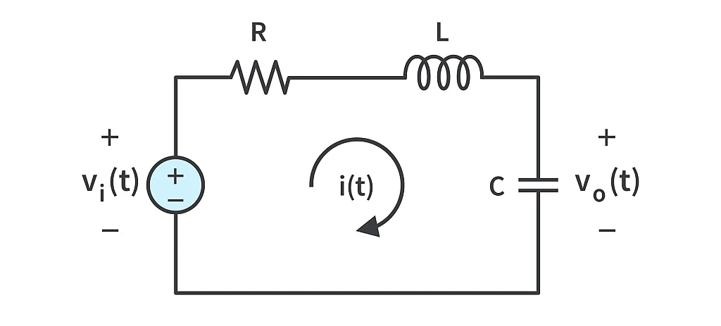
Divide both the numerator and denominator by LC

Now compare this with the standard form of a second order system.

and

If we keep C and L as constant, the damping ratio then depends on the value of resistance.

So, let’s fix C = 1F and L = 1H for simplicity.

Hence,

Now, we shall see all the cases with the help of LTSpice (Check out this tutorial on Introduction to LTSpice by Josh).

First, R = 0, which means ζ = 0 (undamped case)

Please note, the red waveform is the response while the green one is the input.

Next, R = 1, which means ζ = 0.5 (underdamped case)

Next, we take R = 2 implying ζ = 1 (critically damped case)

Finally, we take R = 4 which means ζ = 2 (overdamped case)

These exactly match with what we discussed previously. You can also rig up this circuit and connect an oscilloscope with a square wave input and slowly varying the resistance could make us see the beautiful transition of a system from being undamped to overdamped.

Coming to the end of this lengthy tutorial, it is worth noting that most practical systems are underdamped. In real life it is extremely difficult to design a system that is critically damped. It’ll always end up either being underdamped or overdamped. For an overdamped system, we will never know if the system reached a steady state or not and for this reason, most practical systems are made to be underdamped. You can consider your door damper as an example which is used to slow down the doors. If it's overdamped, we’ll never know if the door has shut fully. Making it slightly underdamped will ensure that the door closes fully with a very small amount of slamming.

To summarize - In this tutorial we learned the standard form of second order systems and various damping conditions. Then we moved towards understanding the impulse response of second order systems for various damping conditions and similarly with the step response. Later on, we took an example of an RLC circuit and verified the step response for various cases of damping. At last, we understood why practical systems are underdamped.

In the next tutorial, we shall continue our journey with time response analysis by learning about certain time domain specifications. Thanks for reading!