Routh-Hurwitz Criterion for Stability Part 2 | Control Systems 3.3
Published
In the last tutorial, we started with the Routh Hurwitz Criterion to check for stability of control systems. We ended the last tutorial with two characteristic equations. As was mentioned, there are equations on which we will get stuck forming the routh array and we used two equations as examples. These are the special cases of Routh Hurwitz Criterion. In this tutorial, we shall start with understanding the special cases, then we’ll see how to use the RH Criterion to design control systems and finally we’ll learn how all these calculations can be avoided with Scilab with a few lines of code.
Let’s take the first characteristic equation that was mentioned at the end of the last tutorial.
Special Case 1

We shall now form the routh array for the characteristic equation above using steps that we learned in the last tutorial.
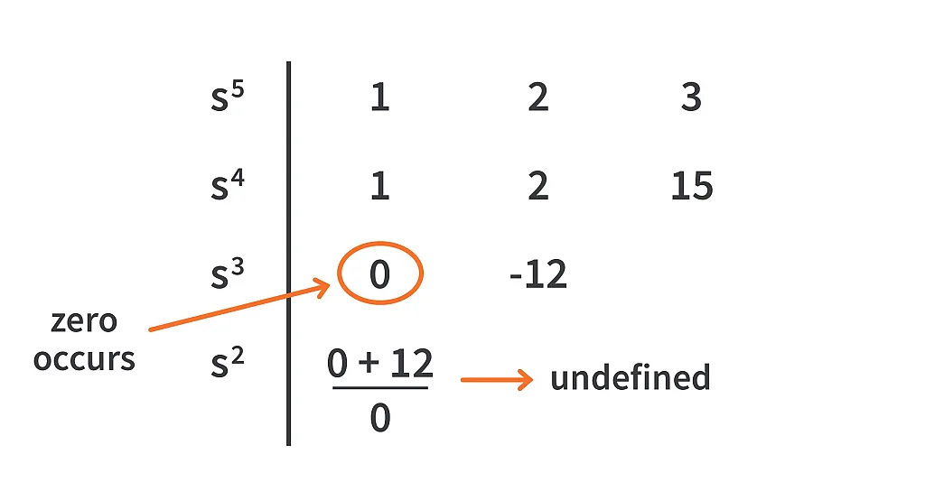
As seen, the first element of the third row becomes 0 and due to this, the first element of the next row is undefined. So, what do we do?
Here’s the solution - if the first element of any row in a Routh array becomes zero, then the zero is replaced by a small positive number which is usually represented by ϵ (pronounced as epsilon).
Now, to evaluate the stability, the sign of the first element of the corresponding rows is found by making ϵ approach zero. Then the sign changes are looked for analysing stability as usual. The example below will make it clear.
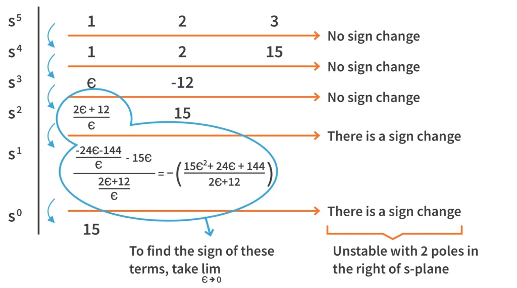
As you can see, when ϵ → 0, the first element of the fourth row is positive and that of the fifth row is negative. As one of the elements of the first column is negative, the system is unstable and as there are two sign changes, there are two poles in the right half of the s-plane.
Special Case 2
Let’s now take the second characteristic equation that was mentioned at the end of the last tutorial.

Forming its Routh array,
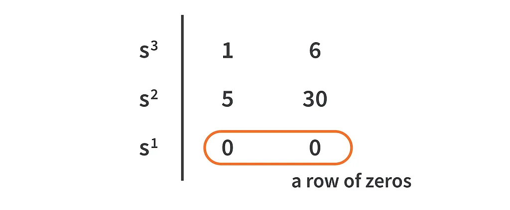
The entire third row becomes zero and due to this, we can’t proceed further and form the fourth row. So, what do we do now?
In this case, we take the polynomial formed by the row above the row of zeros (this polynomial is known as an auxiliary polynomial) and then differentiate with respect to s. The row of zeros is then replaced by the coefficients of the polynomial obtained after differentiation. The example will make it clear.
The second row is taken to form the auxiliary polynomial.


Now, replace the zeros of the third row with 10 and 0 and proceed as usual.
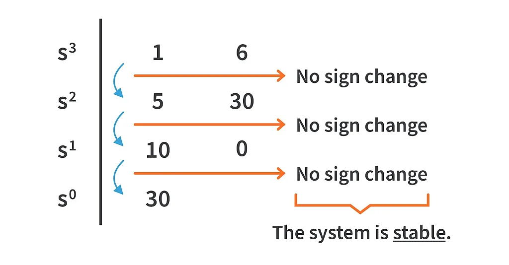
Since all the elements in the first column are positive the system is stable. To be more accurate, the system is marginally stable due to the occurrence of a row of zeros. Here’s why.
The auxiliary polynomial is a polynomial whose roots are symmetric about the origin in the s-plane.
This occurs under three conditions.
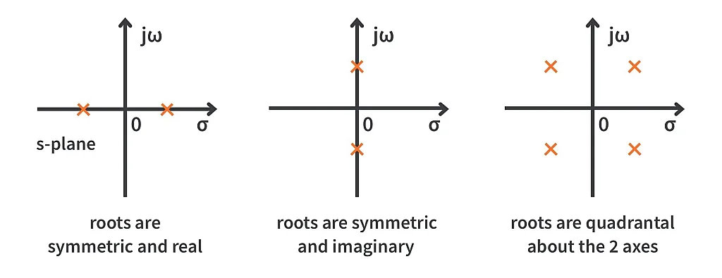
On solving the auxiliary polynomial obtained in the previous example,


And as there are roots on the imaginary axis, we conclude that the system is marginally stable.
Try this by yourself,
Check for stability of the system whose characteristic equation is given by,

Solution:
Routh array
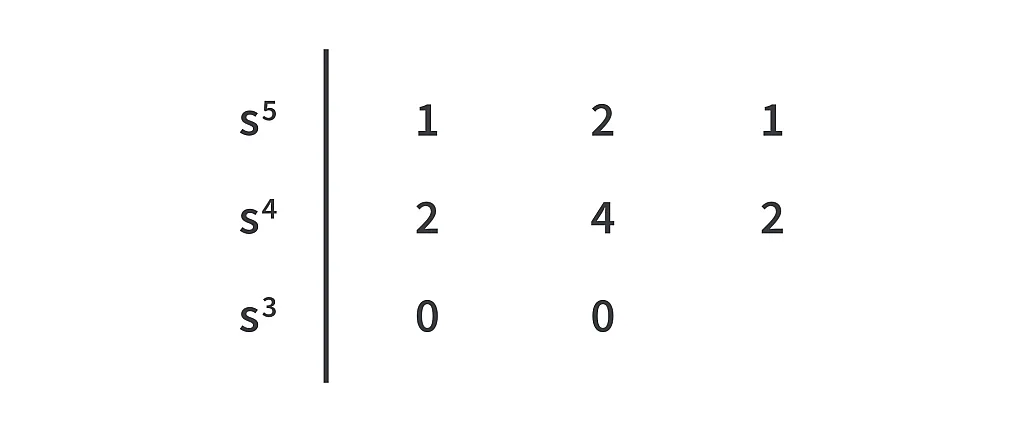
Since the entire 3rd row is zero, the auxiliary polynomial is given by


Replacing the zeros in the third row by 4, 4 and 0 and continuing as usual, the Routh array becomes.
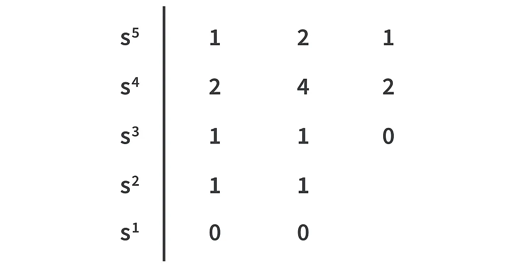
Now again, the entire 5th row is zero, so we form an auxiliary equation again.


Replacing the zeros in the fifth row by 2 and 0 and proceeding as usual, we get the Routh array as follows.
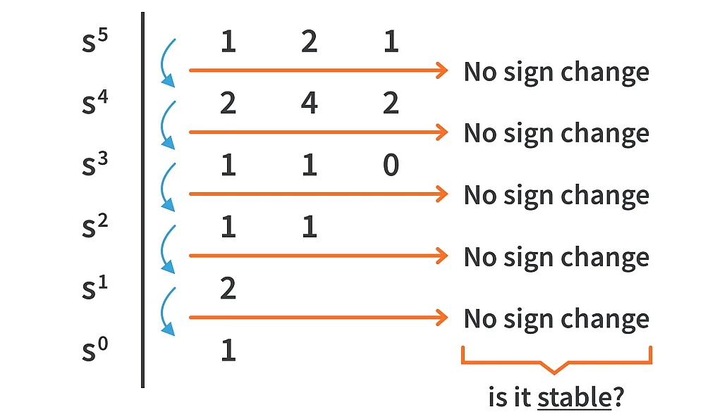
You might think that since all the elements in the first column of the Routh array are positive, the system is stable. But it’s wrong. Here’s why.
Solving the first auxiliary equation, we get


And now solving the second auxiliary equation, we get


There are repeated poles on the imaginary axis. If you can recall from tutorial 3.1, the system becomes unstable if there are repeated poles on the imaginary axis. Hence, the system described in the example above is unstable.
Practical Example of Creating Stable Systems
Covering those special cases, we can now move ahead and learn how we can design stable systems. For this, we shall take an example.
Consider a system with an open loop transfer function

where K is positive.

Let’s find it’s closed loop transfer function.

The characteristic equation

The Routh array for the above system becomes.
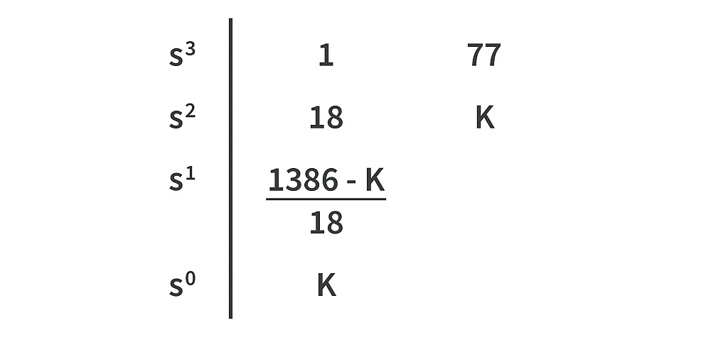
 and
and  that is
  .
.For the system to be stable, design should be such that
If 
If 
With Scilab, life is much easier.
Consider a large characteristic equation:

Let’s use Scilab to obtain the routh array.

And the output

As you can see, there are two sign changes, so the system is unstable. But it’s much easier than doing the calculations by hand.
Summary
To summarize – in this tutorial, we discussed two of the special cases in the Routh Hurwitz Criterion. Then we learned how the RH criterion can be applied during the design of control systems and finally we used Scilab to compute the Routh array of a big characteristic equation. Although the Routh Hurwitz Criterion gives a good understanding of the stability of the system, it doesn't tell us the exact location of the poles. Hence, in the next tutorial we shall start understanding the root locus plot which gives us a good visual representation of the system’s stability.

Get the latest tools and tutorials, fresh from the toaster.


