The Concept of Stability | Control Systems 3.1
Published
In the previous chapter, we learned about the time response analysis of control systems. Starting with this tutorial, we shall discuss the stability of control systems. We shall begin this chapter by introducing the concept of stability with respect to control systems.
Let’s start by defining stability.
A system is said to be stable if the system eventually returns to its equilibrium state when the system is subjected to an initial excitation or disturbance.
If the response of a system diverges without bound from its equilibrium state up on excitation, then its unstable.
Here is a classic example to introduce the concept of stability.
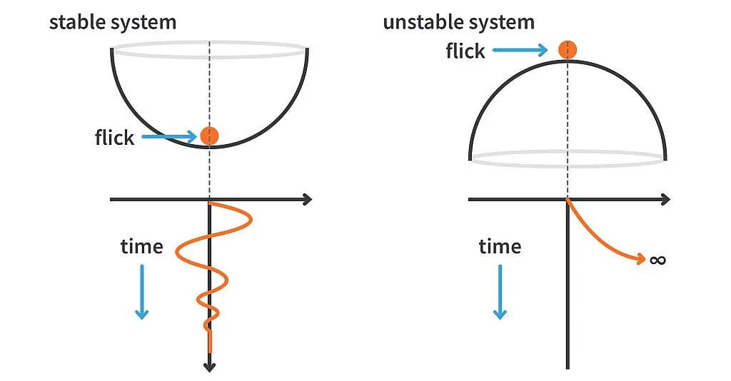
Consider a marble and a bowl arranged as shown above. In the first case, the marble is inside the bowl. A small flick will make the marble oscillate about its equilibrium position and it will eventually settle back to its original position. In the second case, the marble is placed on top of an inverted bowl. A small flick in this case would make the marble fall off the bowl and the marble would never come back to its initial position unless you take it and place it back.
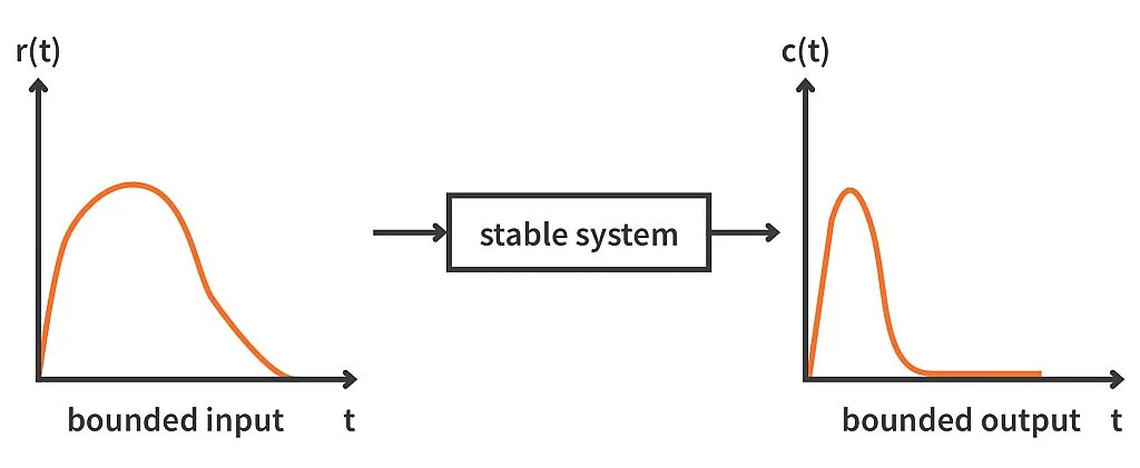
Now, let’s come back to the first case where the marble is inside the bowl. What if I flick the marble so hard that it flies out of the bowl? Will the marble come back to its initial position? It’s an obvious NO. So, is the system unstable? The system is stable, but exciting it with an unbound input makes it difficult to judge if the system is stable or not. This brings us to the concept of the bounded input. An input is said to be bounded if the input lies within definite limits of the system. If it’s not bounded, then the input is an unbounded input. As simple as it sounds.
Based on this, let’s note a few points:
1. For every bounded input signal, if the system response is also bounded, then that system is stable.
2. For any bounded input, if the system response is unbounded, then that system is unstable.
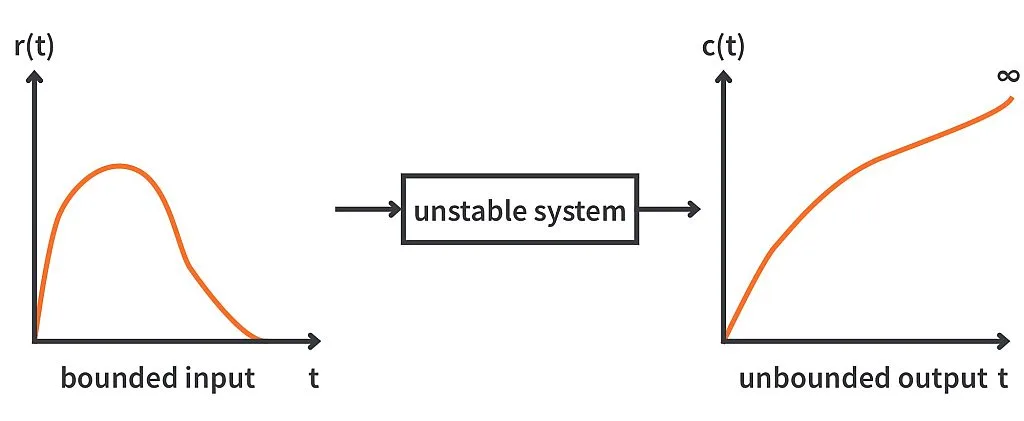
This is commonly called as BIBO Stability meaning – Bounded Input Bounded Output Stability.
With this idea on stability, we shall move ahead to poles and zeros which we have discussed earlier.
A transfer function G(s) of a system can be represented as the ratio of two polynomials.

Here, the poles of the system are the roots of the denominator polynomial D(s) (poles are the values of s for which D(s) is zero) and the zeros of the system are the roots of the numerator polynomial N(s) (zeros are the values of s for which N(s) is zero). Hence, in the generalised equation shown above, the system has n poles and m zeros.
Let’s see an example,
Consider a system with transfer function,

Solving N(s) and D(s), we get
Zeros as -1.5 ± 3.1225j
Poles as -2, -3
Now, with the help of Scilab, we shall view its pole – zero plot in the s-plane.
Have a look at this code, it is very simple.
s = %s;    // defines 's' as polynomial variable
tf = syslin('c', s^2 + 3*s + 12, s*(s^2 + 5*s + 6));    // defining the transfer function. This syntax is - syslin('c', numerator, denominator) where 'c' denotes the continuous time
plzr(tf) //this produces a pole - zero plot of the transfer function tf

Now, we shall explore the effect of location of poles on the stability of the control systems. We shall split this into several cases to make it clear.
Case 1 – Poles on the negative real axis.
Consider a simple pole at s = -2
This means the transfer function would be

With Scilab,
s = %s;    // defines 's' as polynomial variable
tf = syslin('c', 1, s+2);    // defining the transfer function. This syntax is - syslin('c', numerator, denominator) where 'c' denotes the continuous time
plzr(tf) //this produces a pole - zero plot of the transfer function tf
t = 0:0.0001:5;            // setting the simulation time to 5s with step time of 0.0001s
c = csim('imp', t, tf);    // the output c(t) as the impulse('imp') response of the system
figure
plot2d(t, c)
xgrid (5 ,1 ,7)            // for those red grids in the plot
xtitle ( 'Impulse Response', 'Time(sec)', 'C(t)')
And we get pole zero plot and impulse response as,


As we can see, with time, the response approaches zero and the system is stable.
Case 2 – Poles on positive real axis
Consider a simple pole at s = 2
This means the transfer function would be

With Scilab, just change the transfer function in the previous code. The pole zero plot and impulse response obtained is


The response increases exponentially, and this means that the system doesn’t settle, and it is marked as unstable.
Case 3 – Poles at origin
First, consider one pole at origin. The corresponding transfer function would be

By changing the transfer function in the previous script, we obtain the pole zero plot and impulse response as


As we can observe, the impulse response stays constant at 1 as time progresses. If the response slightly decreases with time, then it eventually settles at zero and the system can be called stable. If the response slightly increases with time, the response increases to infinity eventually and the system is marked unstable. So, this response where the slightest variation changes the stability of the system is the response of a marginally stable system. Hence, the example shown in this case is marginally stable.
Next, we consider two poles at origin. The corresponding transfer function becomes,

By changing the transfer function in the previous script, we obtain the pole zero plot and impulse response as


As it is seen, with multiple poles at origin, the response increases without bound and hence the system is marked unstable.
Case 4 – Complex pole in the left half of s-plane
Consider a complex pole pair at s = -2+3j and at s = -2-3j
The corresponding transfer function would be,

By changing the transfer function in the previous script, we obtain the pole zero plot and impulse response as


As the response approaches 0 as time increases, the system is stable.
Case 5 – Complex poles in the right half of the s-plane
Consider a complex pole pair at s = 2+3j and at s = 2-3j
The corresponding transfer function would be,

By changing the transfer function in the previous script, we obtain the pole zero plot and impulse response as


As seen, the oscillation of the response keeps growing in amplitude and hence the system response becomes unbound and unstable.
Case 6 – Poles on the imaginary axis
The poles lying on the imaginary axis are purely imaginary. Consider the poles to be at s = 3j and at s = -3j.
The corresponding transfer function would be,

By changing the transfer function in the previous script, we obtain the pole zero plot and impulse response as


The response for this type of system is a sustained oscillation (an oscillation where the amplitude remains constant with time). Now if the amplitude of the oscillation slightly reduces, it eventually decays with time. But if the amplitude of the oscillation slightly increases, it eventually rises to infinity with time. The condition where in the response is a sustained oscillation, lies in between being stable and unstable. Hence, such systems producing a sustained oscillation are marginally stable.
Let’s conclude a few points based on the cases discussed above.
- If all the poles lie in the left half of the s-plane, then the system is stable.
- If any pole lies in the right half of the s-plane, then the system is unstable
- If the system has two or more poles in the same location on the imaginary axis, then the system is unstable.
- If the system has one or more non-repeated poles on the imaginary axis, then the system is marginally stable.
To summarize - In this tutorial, we started with the next step in our journey with control systems by introducing ourselves to the concept of system stability with an example of a bowl and a marble. Next, we revisited the pole zero form of a transfer function, and then learned about the effect of location of poles on the stability of control systems.
In the next tutorial, we shall look at some of the methods to determine the stability of control systems.

Authored By
Kushal Gowda
An Electrical and Electronics Engineer. Loves playing Table Tennis, Cricket and Badminton . Always ready to learn and teach. His fields of interest include power electronics, e-Drives, control theory and battery systems.

Related Tutorials

Explore CircuitBread
- 244 Tutorials
- 9 Textbooks
- 12 Study Guides
- 31 Tools
- 104 EE FAQs
- 295 Equations Library
- 213 Reference Materials
- 97 Glossary of Terms
Friends of CircuitBread
-

Free Educational Blog Content
-

Free Electronics Lessons & Resources + 2 Perks
-

Partner Store With Academic Discount Pricing


Get the latest tools and tutorials, fresh from the toaster.


