Proportional, Integral, and Derivative Control | Control Systems 4.2

In the last tutorial, we understood the basics of the operation performed by a controller or a compensator. In this tutorial, we shall learn about the “Proportional, Integral and Derivative Control” (PID Control) which is probably one of the most widely used control techniques.

A general block diagram of a system with PID Control is as shown below,

We shall start with proportional control and go over each type one by one.

The proportional control acts on the current error, that is, it gives the control action which is proportional to the error present. To make it clear, let’s take a general example. Suppose you want to walk starting from point A and your destination is point B. Once you start walking, the error (difference between the desired position and the current position) is large and hence, you walk faster. But as you approach point B, you start slowing down and you eventually stop walking when you are at point B. In this case, your speed is directly proportional to the error. This way of controlling your speed based on the error is nothing but proportional control.

Consider a first-order plant with proportional control as shown below,

The open loop transfer function for the plant above is

and the closed loop transfer function is

For a unit step input as reference, let’s find the steady state error that the plant produces.

The error is given by E(s),

The steady state error e_ss is given by

From these equations, we can observe that with the inclusion of proportional control, the time constant of the system has reduced from T to

which means the system responds much faster now.

Another observation is that the steady state error is reduced as we increase K_p, but increasing K_p in higher order systems as we saw in the tutorial on root locus plot, takes the poles to the right half of the s plane making the system unstable.

For this tutorial we shall use Scilab’s XCOS as our simulation tool. It has a built-in PID block which makes it simpler for us.

Let’s create the block diagram.

When you click on the PID control block, this window opens.

Here you can set the parameters.

First to simulate without the proportional control, we make K_p = 1 and keep others 0.

The response we get is

As we see, there is a large steady state error. (The green one is the response and the black one is the reference input)

Let’s simulate with proportional control and for this, we shall set K_p = 20 and keep others 0.

The response we get is

The system now responds faster as well as the steady state error is reduced which proves what we discussed earlier.

Integral control acts on the accumulated error and not the current error. This means that even if the error becomes zero after a certain time, the control action doesn’t become zero but remains constant. An example for this would be a helicopter or a drone. Say you want to rise to a height of X meters from ground, once it rises to that height, you want to maintain that speed of the propellers constant and not turn them off. As the error becomes less, the speed of the propellers saturates and becomes constant. In this type of situation, you use an integral.

Consider a first order plant/system with integral control as shown below,

The output of the controller is the integral of the error signal.

Which is nothing but

The open loop transfer function for the plant above is

and the closed loop transfer function is

As we did earlier, we shall compute the steady state error for a unit step input as reference.

The error is given by E(s),

The steady state error e_ss is given by

With the integral control, we are now able to completely make the steady state error 0, but this comes at a cost of increasing the order of system (originally the system in this example was of first order, but with integral control, <em>G(s)</em> is second order), and we have seen in the tutorial on root locus that adding an open loop pole to a higher order system can make the system unstable. Hence, there is this risk. Most of the time, integral control is used along with proportional control, and it’s called proportional – integral control. We shall come to the reason for this shortly.

To simulate this, we take the same block diagram, but here we set K_i = 1 and all others 0.

Let’s look at the response,

The steady state error here is 0 and as the order of the system has increased to two now, we see a slight oscillation initially which supports our discussion.

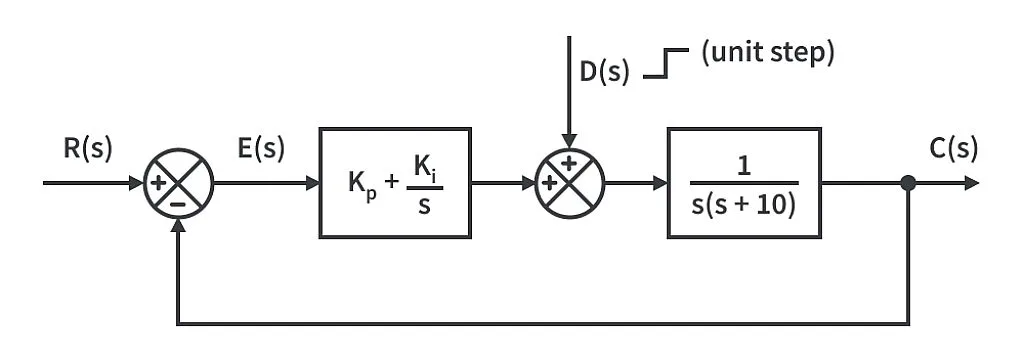
Let’s now consider a second order system,

and given below is a block diagram of the system with proportional control with an external disturbance D(s)

Let’s now compute the transfer function relating disturbance D(s) to the output C(s) by setting input R(s) to 0.

Now the error E(s) is given by,

If we assume D(s) to be a unit step function, then

The steady state error will be

Let’s build this block diagram first,

Here, to make steady state error much smaller, we shall make K_p = 1000 and see the response.

Although steady state error has been reduced to almost zero, we see high frequency oscillations at the start. Hence, the steady state can be reduced by increasing K_p but the tradeoff is that the system starts becoming more oscillatory (higher natural frequency) and this may affect the stability.

Now we shall include Integral control along with the proportional control in the same system and see how things change from before.

Let’s now compute the transfer function relating disturbance D(s) to the output C(s) by setting input R(s) to 0.

Now the error E(s) is given by,

If we assume D(s) to be a unit step function, then

The steady state error will be

Here, we should choose K_p and K_i such that the system is stable. Let’s use the Routh array.

For stability,

Let’s choose K_p = 10 and K_i = 20 (as 10 * 10 > 20) in this example to obtain observations simulating this example.

Hence, we can say that the proportional and integral control together did a good job in eliminating the steady state error while not being too oscillatory. The PI (proportional-integral) control does a good job in rejecting the disturbance.

Why can’t we just use the integral control in this case?

Let’s see.

For the above system, the open loop transfer function becomes

This now has two poles at origin. If you can remember, we had discussed that if there are overlapping poles on the imaginary axis of the s-plane, then the system inherently becomes unstable. If you don’t remember, it’s fine. We can just simulate it and check. Let’s take K_i = 10 as an example in this case.

Hence, in this case proportional control along with the integral control is necessary. While the integral control removes the steady state error, the proportional control tries to keep the system stable.

The derivative control acts on the rate of change of the error signal or in other words the control action is proportional to the rate of change of the error signal. Let’s understand with an example.

Consider the plant with a proportional control as shown below.

The closed loop transfer function of the above system is

Whatever the value of K_p , this system is purely oscillatory as it is marginally stable (has poles on the imaginary axis) for a step input. Let’s take K_p = 10 to simulate and check.

The block diagram,

The response,

As we see, this has undamped oscillations. We need our controller to somehow damp these oscillations and this job is done with the derivative controller.

We’ll incorporate derivative control in the previous example.

The output of the controller is

and taking the inverse Laplace transform of it,

As we discussed, the control action now depends on the rate of change of error.

The closed loop transfer function of the system now becomes

Now this is always stable given that K_d and K_p are greater than 0. For simulation, we shall take K_d = 5 and K_p = 10.

This gives

which means the system is slightly underdamped and hence we should see a slight overshoot.

The response,

This response supports what we discussed.

Even the derivative control is not used independently. It's always used with proportional control (proportional – derivative control). This is because when a system is having a constant error, the derivative of it will give zero and this will make the system output zero and we don’t want that to happen.

Next, to learn proportional-integral-derivative control (all of them together) and to summarize, we shall take an inherently unstable system and try to obtain the desired response from it.

The response of this system for a step input is as follows,

Clearly, this is unstable.

As one of its poles,

lies in the right half of the s-plane, the system is unstable.

We shall use the unit step input as the reference throughout this example.

Let’s start with only proportional control and see if we can stabilize it to the desired output.

The closed loop transfer function becomes,

This system can be brought from being unstable to being marginally stable if we make K_p > 10. So we choose K_p = 20 and check by simulating it.

The block diagram,

The response,

Clearly, we can’t stabilize the system only with proportional control. Since we need to damp out the oscillations here, we shall add derivative control.

The closed loop transfer function now becomes,

This will be stable for K_p > 10 and K_d > 0, so we arbitrarily choose K_p = 20 and K_d = 10 and check the response.

The system seems to be stable now, but there seems to be a large steady state error. To reduce the steady state error, what do we do? We use the integral controller.

Now we shall include the integral controller,

The closed loop transfer function will now be,

For this system to be stable,

Arbitrarily, we choose K_p = 20, K_d = 10 and K_i = 5 making system stable (10 * (20 - 10) > 5) check the response.

As we see, the steady state error is eliminated here, and we have obtained a stable response through PID control. We can achieve even better tracking by properly tuning the parameters K_p, K_d, and K_i . There are few specific methods for tuning these parameters which are beyond the scope of this tutorial series, but still, we can obtain a decent response by tuning them by trial and error.

To summarize, we started with proportional control and then we learnt integral control. We used these both and tried to reject disturbance. Then we learnt about derivative control, then used it along with a proportional control to damp the response. Later we used proportional, derivative as well as integral control to stabilize an unstable system and bring its response close to the desired one by making the steady state error zero. In the next tutorial we shall learn more regarding the PID control.